Table of Contents
Overview
BigQuery can be used to perform more sophisticated data analysis. In this lab, you will analyze soccer event data to achieve real insight from the dataset.
The data used in this lab comes from the following sources:
Pappalardo et al., (2019) A public data set of spatio-temporal match events in soccer competitions, Nature Scientific Data 6:236, https://www.nature.com/articles/s41597-019-0247-7
Pappalardo et al. (2019) PlayerRank: Data-driven Performance Evaluation and Player Ranking in Soccer via a Machine Learning Approach. ACM Transactions on Intelligent Systems and Technologies (TIST) 10, 5, Article 59 (September 2019), 27 pages. DOI: https://doi.org/10.1145/3343172
Objectives
In this lab, you will learn how to:
Analyze soccer event data using various BigQuery features
Write and execute queries that work with nested data in BigQuery tables
Setup and requirements
Before you click the Start Lab button
Read these instructions. Labs are timed and you cannot pause them. The timer, which starts when you click Start Lab, shows how long Google Cloud resources will be made available to you.
This hands-on lab lets you do the lab activities yourself in a real cloud environment, not in a simulation or demo environment. It does so by giving you new, temporary credentials that you use to sign in and access Google Cloud for the duration of the lab.
To complete this lab, you need:
- Access to a standard internet browser (Chrome browser recommended).
Note: Use an Incognito or private browser window to run this lab. This prevents any conflicts between your personal account and the Student account, which may cause extra charges incurred to your personal account.
- Time to complete the lab---remember, once you start, you cannot pause a lab.
Note: If you already have your own personal Google Cloud account or project, do not use it for this lab to avoid extra charges to your account.
How to start your lab and sign in to the Google Cloud console
Click the Start Lab button. If you need to pay for the lab, a pop-up opens for you to select your payment method. On the left is the Lab Details panel with the following:
The Open Google Cloud console button
Time remaining
The temporary credentials that you must use for this lab
Other information, if needed, to step through this lab
Click Open Google Cloud console (or right-click and select Open Link in Incognito Window if you are running the Chrome browser).
The lab spins up resources, and then opens another tab that shows the Sign in page.
Tip: Arrange the tabs in separate windows, side-by-side.
Note: If you see the Choose an account dialog, click Use Another Account.
If necessary, copy the Username below and paste it into the Sign in dialog.
student-02-fe0f402a10eb@qwiklabs.netYou can also find the Username in the Lab Details panel.
Click Next.
Copy the Password below and paste it into the Welcome dialog.
5GT7KBLMOYyMYou can also find the Password in the Lab Details panel.
Click Next.
Important: You must use the credentials the lab provides you. Do not use your Google Cloud account credentials.
Note: Using your own Google Cloud account for this lab may incur extra charges.
Click through the subsequent pages:
Accept the terms and conditions.
Do not add recovery options or two-factor authentication (because this is a temporary account).
Do not sign up for free trials.
After a few moments, the Google Cloud console opens in this tab.
Note: To view a menu with a list of Google Cloud products and services, click the Navigation menu at the top-left.
Task 1. Open BigQuery
The BigQuery console provides an interface to query tables, including public datasets offered by BigQuery.
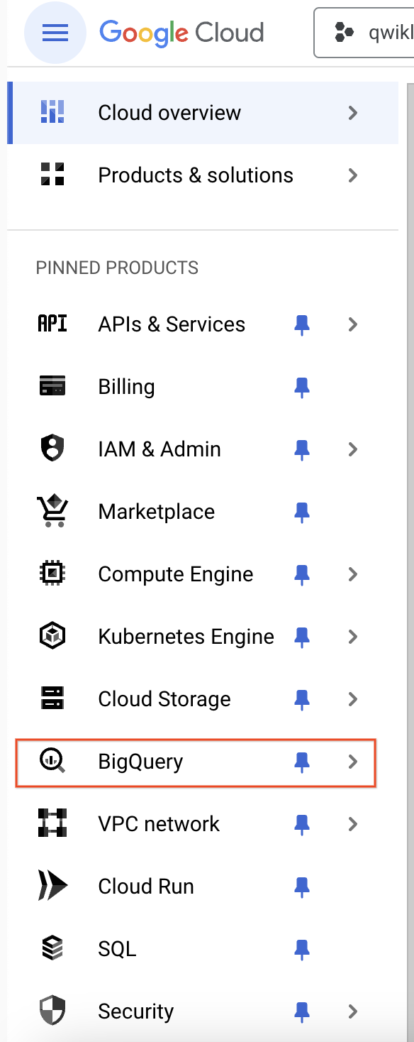
- In the Cloud Console, from the Navigation menu select BigQuery:
The Welcome to BigQuery in the Cloud Console message box opens. This message box provides a link to the quickstart guide and the release notes.
- Click Done.
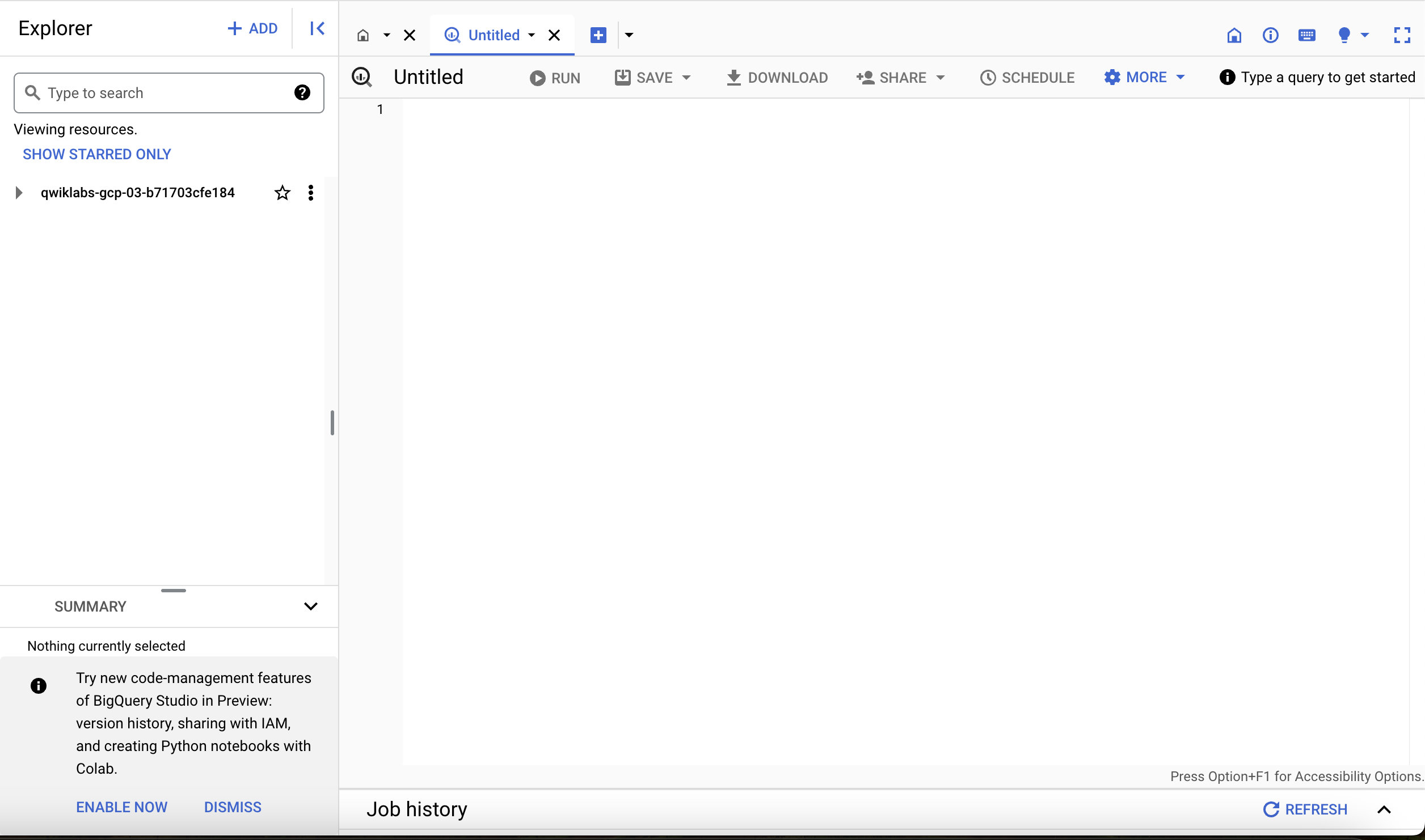
The BigQuery console opens.
Note: The process for creating the dataset and tables is taught in the BigQuery Soccer Data Ingestion lab. In this lab the focus is on learning how to query the information.
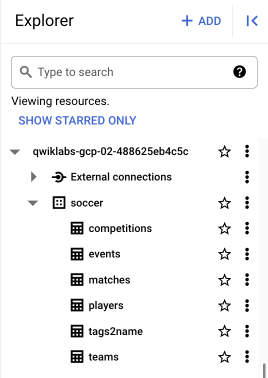
Once the tables are created the display will be similar to below:
In this section the BigQuery interface was used to access the console. The console provides a convenient way to add information to a dataset. BigQuery uses tables to represent data in a structured way.
In the next section learn more about creating more complex queries.
Task 2. Analyze nested soccer event data
In this section, you will run some queries that use JOINs with BigQuery's array functionality to enable better control over the soccer event data.
In the Query editor, click Create SQL query.
Copy and paste the following query into the query Editor:
SELECT
 Events.playerId,
 (Players.firstName || ' ' || Players.lastName) AS playerName,
 SUM(IF(Tags2Name.Label = 'assist', 1, 0)) AS numAssists

FROM
 `soccer.events` Events,
 Events.tags Tags

LEFT JOIN
 `soccer.tags2name` Tags2Name ON
   Tags.id = Tags2Name.Tag

LEFT JOIN
 `soccer.players` Players ON
   Events.playerId = Players.wyId

GROUP BY
 playerId, playerName

ORDER BY
 numAssists DESC
Assists aren't marked as a separate scalar field in the events table, so you need to look "inside" the tags field.
This is done by using a correlated cross join between the events table and the tags field (with the "," in the FROM clause to represent an implicit join) to create 1 row per tag per event (rather than 1 row per event). The tag ID that corresponds to assists is found from the tags2name table, the number of occurrences of that tag is counted by player, and the players table gets player names from their IDs.
- Click Run. The results are displayed below the query window.
Click Check my progress to verify the objective
Check the query has been run
Check my progress
In this section a more complex query was created in BigQuery. Performing Joins in BigQuery and leveraging Arrays provide a powerful way to aggregate data.
In the next section learn how to use Nesting and Arrays with BigQuery.
Task 3. Calculate the average pass distance by team
In this section, you will run some queries that use the nested fields in the soccer event data and BigQuery's array functionality and STRUCT data type to answer some interesting questions.
How much do club teams differ in terms of average distance on their passes (both overall and accurate ones)?
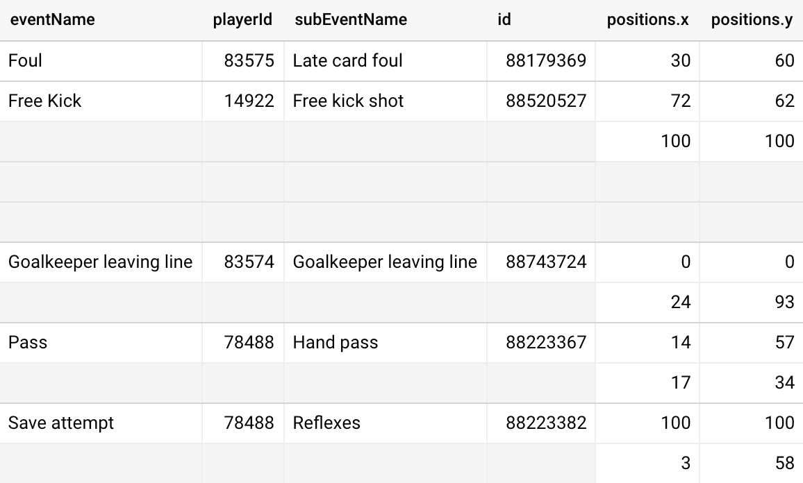
To answer this question, study the positions field in the events table. Observing this data, you see that this is a repeated field that contains 1 or more (x, y) pairs per event. Per Wyscout, a leading data company in the soccer industry that provided this data, these represent the origin and (if applicable) destination positions associated with the event, on a 0-100 scale representing the percentage of the field from the perspective of the attacking team.
The screenshot below illustrates the positions corresponding to a few different event types for a few example events.
From the data you can note that passes have 2 attributes (x, y) pairs representing the start and end position. Therefore pass distance can be calculated by calculating x- and y-coordinate differences, then converting to estimated meters using the average dimensions of a soccer field (105 x 68, per Wikipedia; there is no standard field size) and the 2-dimensional distance formula.
In the Query editor, click Create SQL query.
Add the following query into the query Editor:
WITH
Passes AS
(
 SELECT
   *,
   /* 1801 is known Tag for 'accurate' from tags2name table */
   (1801 IN UNNEST(tags.id)) AS accuratePass,

   (CASE
     WHEN ARRAY_LENGTH(positions) != 2 THEN NULL
     ELSE
  /* Translate 0-100 (x,y) coordinate-based distances to absolute positions
  using "average" field dimensions of 105x68 before combining in 2D dist calc */
       SQRT(
         POW(
           (positions[ORDINAL(2)].x - positions[ORDINAL(1)].x) * 105/100,
           2) +
         POW(
           (positions[ORDINAL(2)].y - positions[ORDINAL(1)].y) * 68/100,
           2)
         )
     END) AS passDistance

 FROM
   `soccer.events`

 WHERE
   eventName = 'Pass'
)

SELECT
 Passes.teamId,
 Teams.name AS team,
 Teams.area.name AS teamArea,

 COUNT(Passes.Id) AS numPasses,
 AVG(Passes.passDistance) AS avgPassDistance,
 SAFE_DIVIDE(
   SUM(IF(Passes.accuratePass, Passes.passDistance, 0)),
   SUM(IF(Passes.accuratePass, 1, 0))
   ) AS avgAccuratePassDistance

FROM
 Passes

LEFT JOIN
 `soccer.teams` Teams ON
   Passes.teamId = Teams.wyId

WHERE
 Teams.type = 'club'

GROUP BY
 teamId, team, teamArea

ORDER BY
 avgPassDistance
The code in the initial WITH clause filters the events table to passes only and adds an accuratePass field by looking "inside" the tags field.
The pass distance is calculated by extracting the initial and final (x, y) coordinates using ORDINAL and applying the concepts and formula mentioned above. The final SELECT statement aggregates the passes data to the team level (filtering to only club teams), including average pass distance on all passes and accurate passes only.
- Click Run. The results are displayed below the query window.
Note: There are some differences in average pass distance across thousands of passes from various teams, going from the lowest average, less than 18 meters (Napoli and PSG) to the highest one, greater than 23 meters (Eibar).
Average accurate pass distance shows similar dispersion, though those values are slightly more compressed across teams.
Click Check my progress to verify the objective
Check the query has been run
Check my progress
In this section BigQuery was used to determine the number of passes and the average distance of passes by team. To achieve this, you used array processing capabilities to extract repeated values in a single field, then calculated the distance between the starting and ending point of each pass.
In the next section learn how to unnest other coordinate data to generate information about shot distances.
Task 4. Analyze shot distance
In this section, you will create a new query to analyze shot distance.
What impact does the distance of a shot have on the likelihood of a goal being scored?
To answer this question use a process similar to the previous section. For shots, use (x, y) values from the positions field in the events table.
Note: As per the previous query, the approximate dimensions of a soccer field are used with the x-coordinate and y-coordinate distances as inputs to the distance formula.
In the Query editor, click Create SQL query.
Copy and paste the following query into the query Editor:
WITH
Shots AS
(
 SELECT
  *,

  /* 101 is known Tag for 'goals' from goals table */
  (101 IN UNNEST(tags.id)) AS isGoal,

  /* Translate 0-100 (x,y) coordinate-based distances to absolute positions
  using "average" field dimensions of 105x68 before combining in 2D dist calc */
  SQRT(
    POW(
      (100 - positions[ORDINAL(1)].x) * 105/100,
      2) +
    POW(
      (50 - positions[ORDINAL(1)].y) * 68/100,
      2)
     ) AS shotDistance

 FROM
  `soccer.events`

 WHERE
  /* Includes both "open play" & free kick shots (including penalties) */
  eventName = 'Shot' OR
  (eventName = 'Free Kick' AND subEventName IN ('Free kick shot', 'Penalty'))
)

SELECT
 ROUND(shotDistance, 0) AS ShotDistRound0,

 COUNT(*) AS numShots,
 SUM(IF(isGoal, 1, 0)) AS numGoals,
 AVG(IF(isGoal, 1, 0)) AS goalPct

FROM
 Shots

WHERE
 shotDistance <= 50

GROUP BY
 ShotDistRound0

ORDER BY
 ShotDistRound0
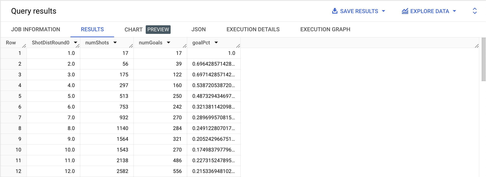
The initial WITH clause filters the events table to shots only, adds an isGoal field by looking "inside" the tags field, and calculates shot distance the same way that pass distance was handled in the previous section, but uses the midpoint of the goal mouth (100, 50) as the ending location.
The final SELECT statement aggregates the number of shots, number of goals, and percentage of goals from shots by distance rounded to the nearest meter.
- Click Run. The results are displayed below the query window.
As expected, shots at close distance have much higher goal rates, going from near 70% success at 2-3 meters down to less than 25% at 8 meters, and declining steadily all the way to 25+ meters.
Create a visualization of results
Visualizing the data can make it easier to understand and see trends.
Click on the CHART in the Query results section.
Select Scatter for the Chart type.
Use the scatter chart creation features in Sheets to create a chart like the one below:
There's a slight bump up in success rate at 11-12 meters, but that can likely be explained by the fact that penalty kicks (which are, by design, much higher propositions than most other shots) account for a large percentage of shots from that range.
Click Check my progress to verify the objective
Check the query has been run
Check my progress
In this section BigQuery was used to establish a view on shot distance versus goal success rate. From this analysis there is a better understanding of the likelihood of a goal being scored based on the distance of the shot.
In the next section you will perform a similar analysis to look at the impact of shot angle on shot success.
Task 5. Analyze shot angle
In this section, modify the previous query to look at the impact of the angles on shots.
In this case, the angle calculated is the one made by the location of the shot and the goal line, as shown below (image credit to Ian Dragulet).
Larger angles arise from being close to the goal and in the center, so this is somewhat correlated with the distance calculation performed above. The shot angle calculations involve using BigQuery's trigonometric functions on the (x, y) data.
In the Query editor, click Create SQL query.
Add the following query into the query Editor:
WITH
Shots AS
(
 SELECT
  *,

  /* 101 is known Tag for 'goals' from goals table */
  (101 IN UNNEST(tags.id)) AS isGoal,

  /* Translate 0-100 (x,y) coordinates to absolute positions using "average"
  field dimensions of 105x68 before using in various distance calcs;
  LEAST used to cap shot locations to on-field (x, y) (i.e. no exact 100s) */
  LEAST(positions[ORDINAL(1)].x, 99.99999) * 105/100 AS shotXAbs,
  LEAST(positions[ORDINAL(1)].y, 99.99999) * 68/100 AS shotYAbs

 FROM
   `soccer.events`

 WHERE
   /* Includes both "open play" & free kick shots (including penalties) */
   eventName = 'Shot' OR
   (eventName = 'Free Kick' AND subEventName IN ('Free kick shot', 'Penalty'))
),

ShotsWithAngle AS
(
 SELECT
   Shots.*,

   /* Law of cosines to get 'open' angle from shot location to goal, given
    that goal opening is 7.32m, placed midway up at field end of (105, 34) */
   SAFE.ACOS(
     SAFE_DIVIDE(
       ( /* Squared distance between shot and 1 post, in meters */
         (POW(105 - shotXAbs, 2) + POW(34 + (7.32/2) - shotYAbs, 2)) +
         /* Squared distance between shot and other post, in meters */
         (POW(105 - shotXAbs, 2) + POW(34 - (7.32/2) - shotYAbs, 2)) -
         /* Squared length of goal opening, in meters */
         POW(7.32, 2)
       ),
       (2 *
         /* Distance between shot and 1 post, in meters */
         SQRT(POW(105 - shotXAbs, 2) + POW(34 + 7.32/2 - shotYAbs, 2)) *
         /* Distance between shot and other post, in meters */
         SQRT(POW(105 - shotXAbs, 2) + POW(34 - 7.32/2 - shotYAbs, 2))
       )
     )
   /* Translate radians to degrees */
   ) * 180 / ACOS(-1)
   AS shotAngle

 FROM
   Shots
)

SELECT
 ROUND(shotAngle, 0) AS ShotAngleRound0,

 COUNT(*) AS numShots,
 SUM(IF(isGoal, 1, 0)) AS numGoals,
 AVG(IF(isGoal, 1, 0)) AS goalPct

FROM
 ShotsWithAngle

GROUP BY
 ShotAngleRound0

ORDER BY
 ShotAngleRound0
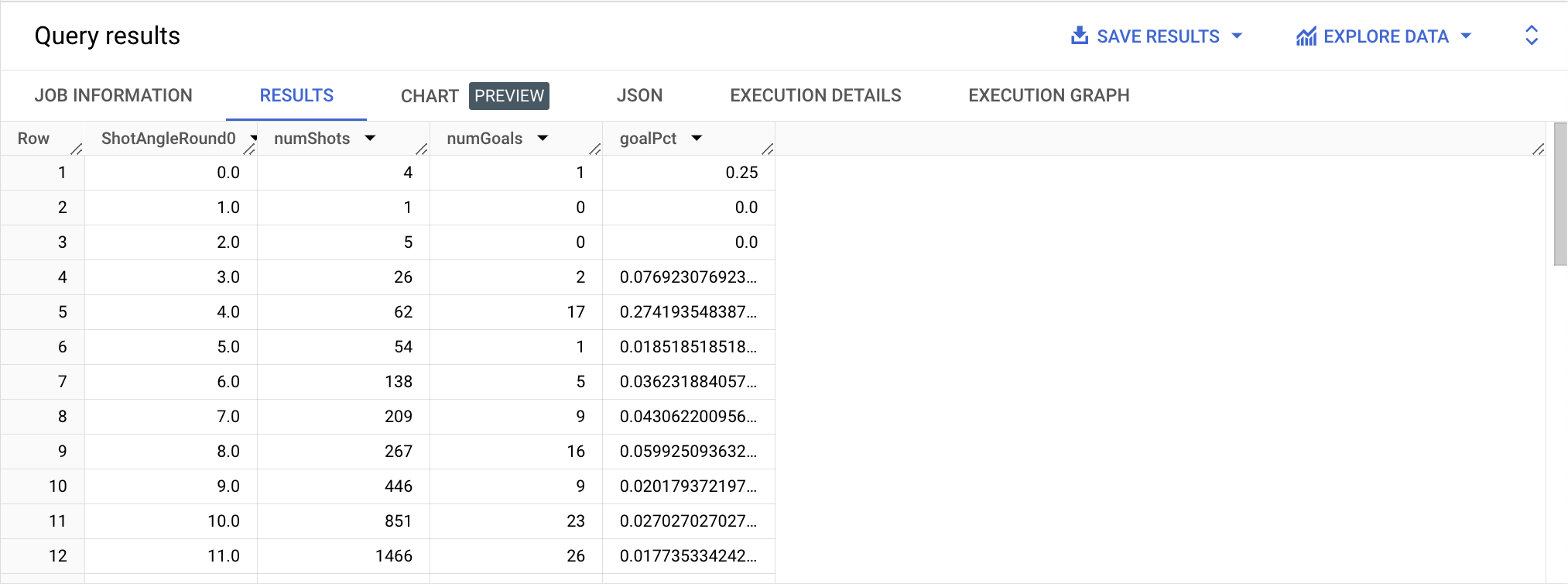
This query is similar to the shot distance one above except for an initial WITH clause to extract the shot coordinates (to simplify when needing them multiple times in the angle calculation) and a more detailed trigonometric calculation using the Law of Cosines to get shot angle in the second WITH clause.
The final SELECT statement aggregates by shot angle rounded to the nearest degree.
- Click Run. The results are displayed below the query window.
Shot angle seems to be generally positively correlated with goal success rate, going from single-digit success rate at angles below 20° to much higher rates at wider angles (with relatively lower sample sizes beyond 60° or so).
By clicking on the Charts in the Query results section, selecting Scatter for the chart types, and then you can visualize the full trend like you see below.
The plot shows that the relationship between shot angle and success rate is relatively linear up to about 100°. Again, the widest angles are only possible on shots close to the goal, so some of this is correlated with the distance effect shown above. There is some slight bumping up in success rate at 35° and 38°, as these are the most common shot angles for penalty kicks (again, much higher propositions than most other shots) and account for a large percentage of shots from that range.
Click Check my progress to verify the objective
Check the query has been run
Check my progress
In the next section test your understanding of what you have learned in this lab.
Task 6. Pop quiz
Test your understanding of BigQuery by completing the short quiz on the topics covered in this lab.
How many club teams have an average pass distance less than 20 meters?
18
33
10
How does the distance of a shot affect its likelihood of becoming a goal?
Shot distance seems to be generally positively correlated with goal success rate.
Shot distance seems to be generally negatively correlated with goal success rate.
There is not any correlation between shot distance and goal success rate.
In this data set, at what angle (rounded to the nearest degree) have the most shots been taken?
15°
45°
30°
Solution of Lab
curl -LO raw.githubusercontent.com/quiccklabs/Labs_solutions/master/BigQuery%20Soccer%20Data%20Analytical%20Insight/quicklabsgsp850.sh
sudo chmod +x quicklabsgsp850.sh
./quicklabsgsp850.sh


