Create a Component Anomaly Detection Model using Visual Inspection AI - GSP895
A passionate full-stack developer from @ePlus.DEV
Overview
Visual Inspection AI Assembly Inspection inspects products when components come together during some designated stage of assembling a product. For such inspections, Visual Inspection AI can help you to ensure that components are in the correct location within the overall object, and that each component is not damaged or defective.
PCBs (printed circuit boards) in general are assemblies of components, including through-hole and surface-mounted. Components can be discrete parts placed within the assembly or physical features created within the assembly such as solder joints, glue, or welds. For subassemblies of electronic products, components can be screws, other hardware parts, or whole other subassemblies.
In this lab you will use Visual Inspection AI to prepare a component anomaly detection dataset and then create and train a component anomaly detection model.
Model training can take a long time so this lab is paired with Deploy and Test a Visual Inspection AI Component Anomaly Detection Solution where you deploy a Visual Inspection solution artifact from this lab and then use that artifact to generate inferences about sample images.
Task 1. Identify and detect components
In this task you create a dataset, upload sample images, and select a template image. On the template you will define inclusion and exclusion areas as well as components, then run the alignment task, which will identify the candidate components in each submitted image.
The Assembly Inspection objective is designed for inspecting assemblages of parts. For each part, typically, you need to test that the part:
Is correctly placed in its expected final location, and
It itself is not anomalous or has not been damaged during placement.
In order to define and build an Assembly Inspection objective via the Visual Inspection AI user interface, you need to upload a collection of training images, then define the following through the console:
A template image with bounding box annotations defining where on the template image to find each component, and a string id for each spatial region of each component. Note that a component, such as a screw component, can have multiple regions assigned to it in the case where a component appears in multiple locations.
A set of training images. The Assembly Inspection objective expects most such images to be normal, that is, free of defects. It is, however, possible to specify the NORMAL or ABNORMAL label for a component region in an image when it is known. Since there are many different components in the typical Assembly Inspection image, it is required to specify which region a label applies to - which region illustrates a defective ABNORMAL or non-defective NORMAL example.
Create a dataset
First, create a Dataset.
In the Navigation Menu, click Visual Inspection AI to open the Visual Inspection console.
Click the Enable Visual Inspection AI API button.
Click Check my progress to verify the objective.
Assessment Completed!
Enable Visual Inspection AI API
Check my progress
Assessment Completed!
Click Create a Dataset.
On the Create Dataset page:
For Dataset name enter pcb_component
For Objective select Assembly Inspection.
Click Create.
Dataset creation will take a minute or two to complete.
Click Check my progress to verify the objective.
Create a Dataset
Check my progress
Import training images into the dataset
Now you need to import the training images into the Dataset. You can use the Google Visual Inspection demo dataset. This dataset consists of images of PCB which may be in different locations and orientations. The left image below shows a normal PCB and the right image shows an example of a defect over the component labeled R1 (see blue rectangle near the bottom center of the PCB).
In order to use the demo dataset, you must copy the images to your own Cloud Storage bucket.
- In Cloud Shell, run the commands below to copy images to your Cloud Storage bucket:
export PROJECT_ID=$(gcloud config get-value core/project)
gsutil mb gs://${PROJECT_ID}
gsutil -m cp gs://cloud-training/gsp895/pcb_images/*.png \
gs://${PROJECT_ID}/demo_pcb_images/
Copying will take a few minutes.
- Create a CSV import file using the following commands:
gsutil ls gs://${PROJECT_ID}/demo_pcb_images/*.png > /tmp/demo_pcb_images.csv
gsutil cp /tmp/demo_pcb_images.csv gs://${PROJECT_ID}/demo_pcb_images.csv
Back in the Visual Inspection AI console, on the Import tab, to Select an import file from Cloud Storage, click Browse.
Expand the bucket with a name that matches the lab Project ID.
Select the demo_pcb_image.csv import file.
Click Select.
Click Continue. A status bar will appear to indicate Import in progress.
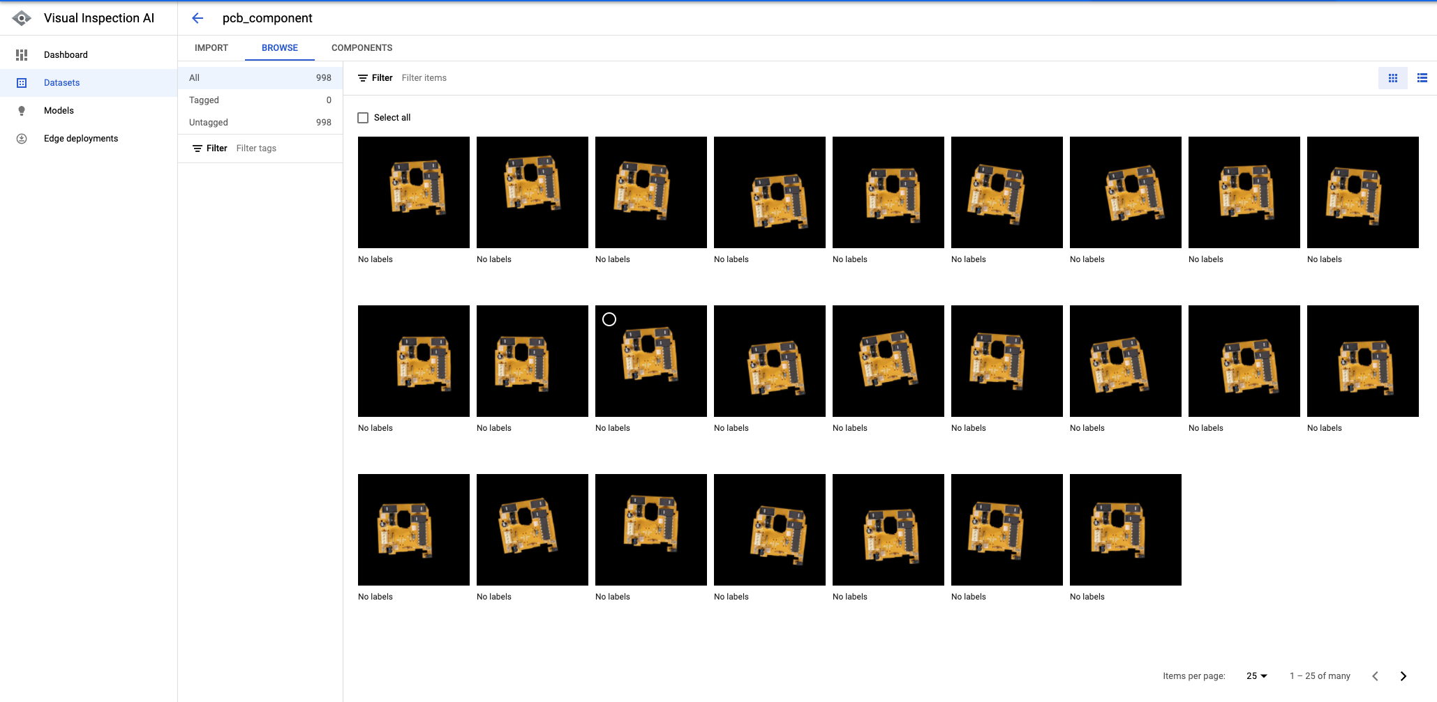
The import will take a few minutes to complete. Once the import is completed, you will see the imported images displayed in the Visual Inspection AI user interface as shown below:
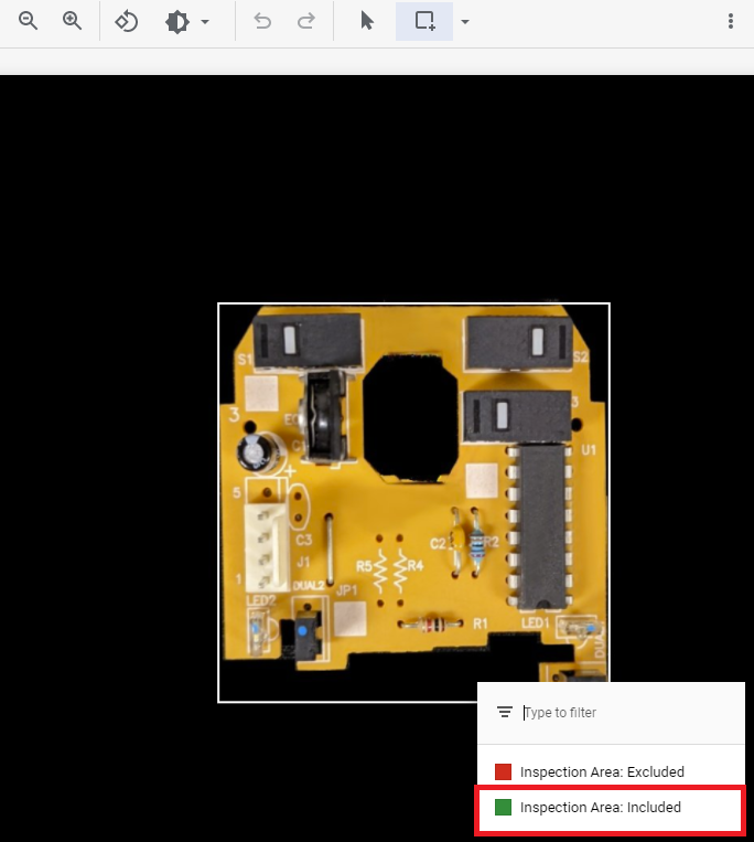
Now that you are able to see the list of imported images, you can browse through them and click any of the images to have a close-up view as you explore your dataset.
Click Check my progress to verify the objective.
Import training images into the dataset
Check my progress
Configure a template
Next, configure a template. To build your Assembly Inspection objective, you will need the following definitions:
Individual components of a to-be-inspected image need to be clearly defined on one template image.
All the individual components from all images localized by the Visual Inspection AI’s algorithms based on the component definition in the template image.
To define an Assembly Inspection objective, you will need to:
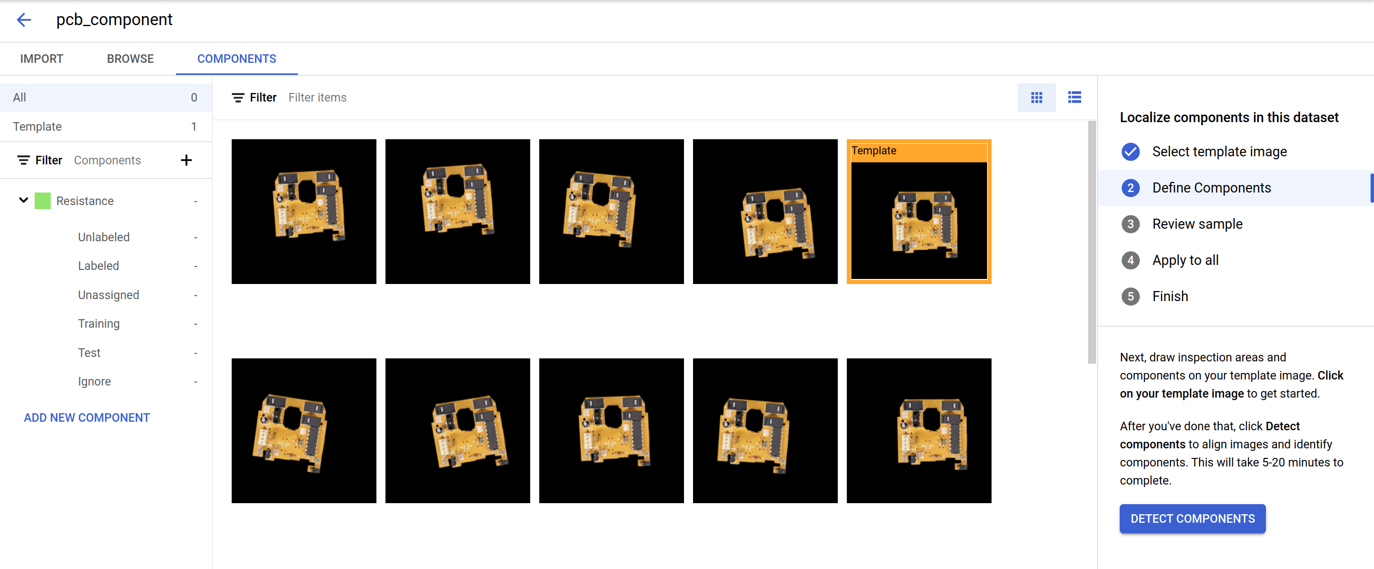
Select one image as the template image from the list of imported images for training.
Define the inspection areas inside the template image, where the subsequent inspection algorithm processes will be applied.
Define individual components with a unique component name and their corresponding spatial locations (or Bounding Box) in the template image.
Select the Components tab in the Visual Inspection AI UI.
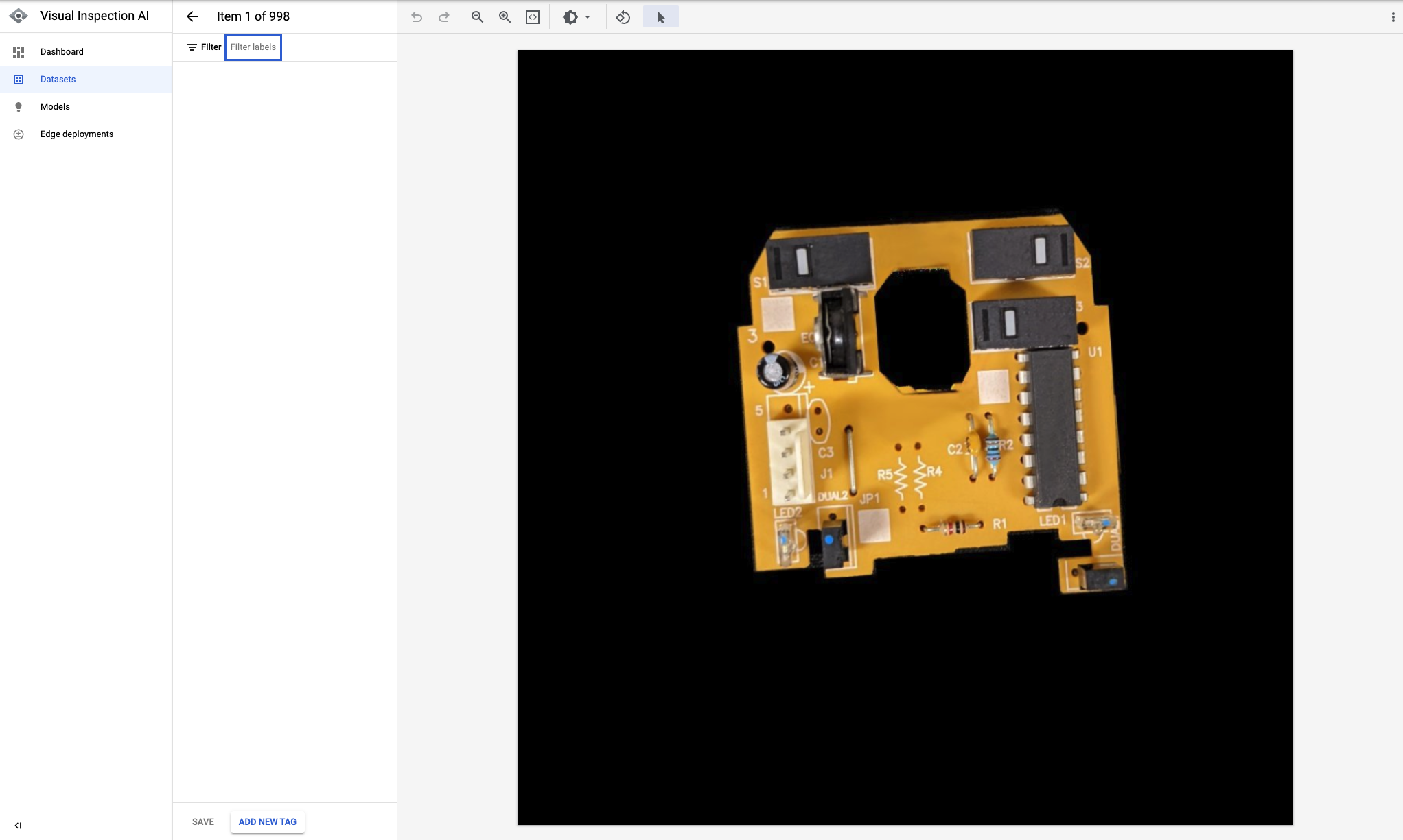
Select one image as the template image by clicking on the image and entering into the zoomed in view.
Toggle the Use as template button as shown below.
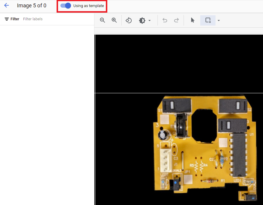
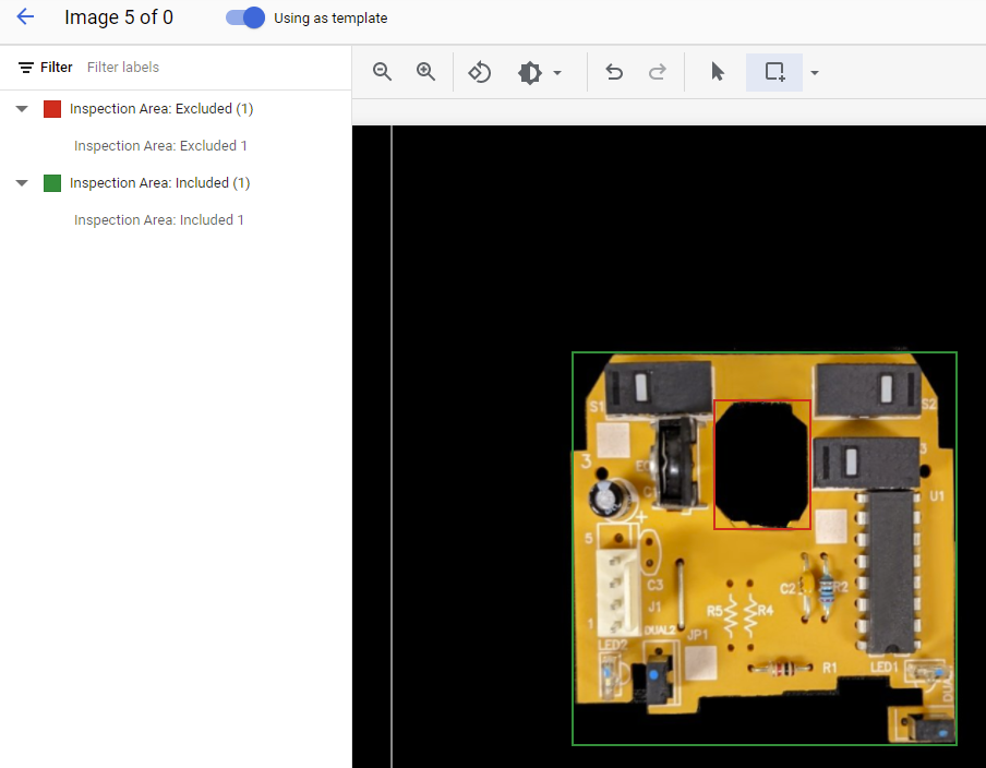
Once the template image is defined, you need to specify an inspection area within the template image where all components to be inspected by the automated algorithm reside. The purpose of defining the inspection area via bounding box regions is to allow the Visual Inspection AI's algorithms to focus only on modeling the pixels that are relevant (Included) and ignore any pixels that are irrelevant (Excluded), such as background pixels.
The following figures show the process of defining the inspection area which has one Included bounding box area and one Excluded bounding box area.
Click the back arrow to return to the Components tab. You will see that the image you selected as the template is now highlighted.
Click the template image to enable selection of inspection areas.
Click the Add bounding box tool from the toolbar and draw a region. When releasing the mouse cursor a popup will allow you to select whether this is an inspection area to include or exclude.
- Click Save.
Detect and crop components via alignment
Once the inspection area is defined, you need to define individual components on the template image for the subsequent component modeling.
You should train Anomaly Detection models for inspecting Resistance components.
You will need to add Resistance components as below:
In the Components tab, click Add New Component.
- For new component name, enter Resistance
Click Done.
Once the component labels are added, you need to associate a concrete component label with a spatial location region within the template image, so that the corresponding image region of the component can be subsequently used for the model training:
Click the Template image for a close-up view.
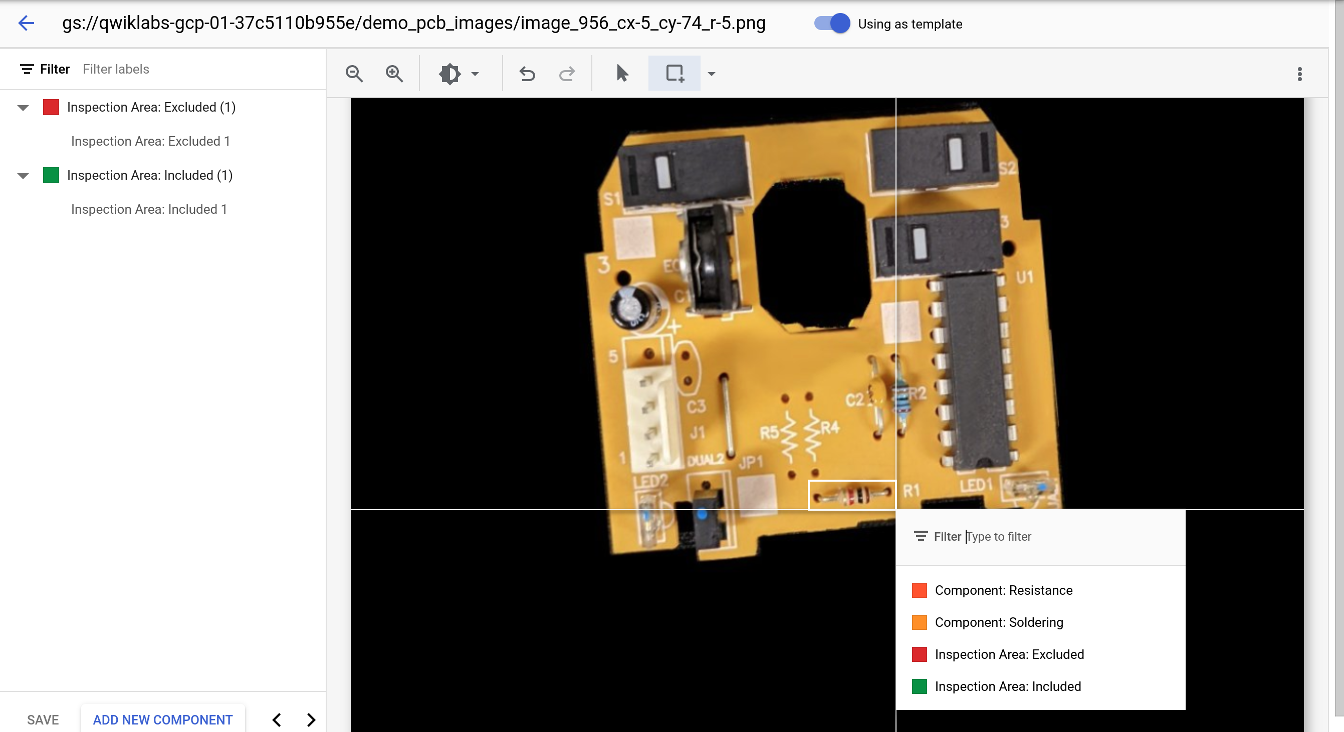
Click the Add bounding box tool from the tool bar.
Draw a region for one Resistance component.
- Select the corresponding component label for the selected region, that is Resistance in the popup menu that appears after releasing the mouse cursor.
Note: You will see Inclusion and Exclusion Inspection Area labels as well as component labels in the popup menu.
Repeat the previous step to select another Resistance component.
Click Save to confirm the component regions.
After defining the template image, inspection areas, and components (labels and regions) on the template image, you can review the detected and cropped component region images.
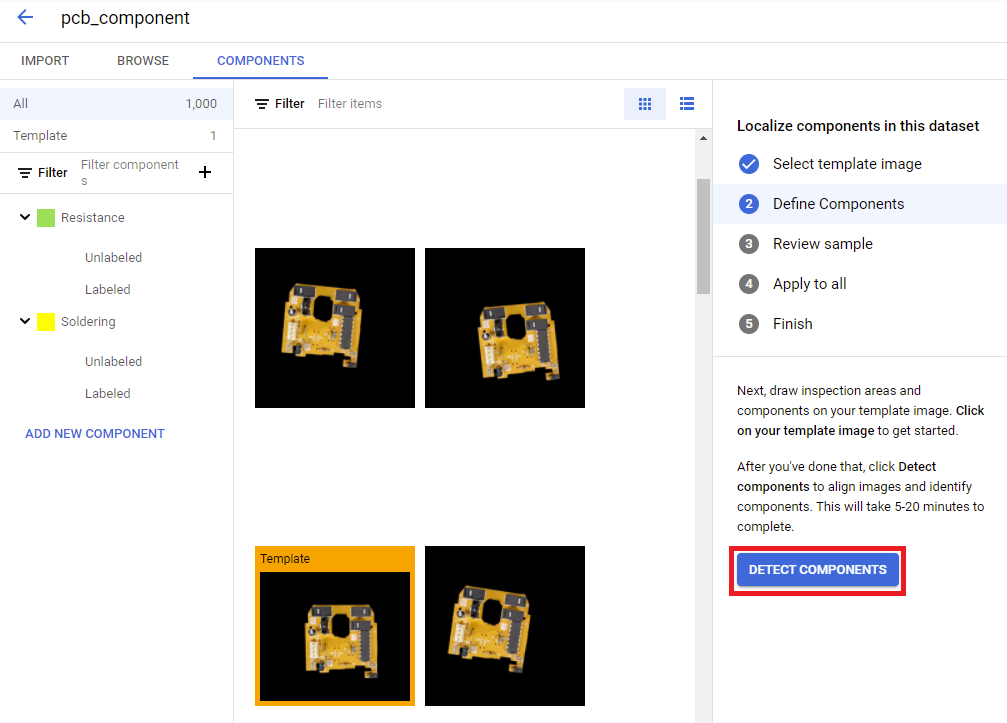
- On the Components tab, on the bottom right, click the Detect Components button.
Note: In the example image below, you will see that there is also a Soldering Component. You do not need to create this component, but you should be aware that model training is per component, and typically you would have more than a single component type. For the purposes of this lab, we will use only the Resistance component type.
Note: The Detect Components task that aligns the images and identifies the components will take about 15-20 minutes to complete.
Task 2. Apply alignment and detection of components
In this task you will apply your component selection to the images to align and detect all components.
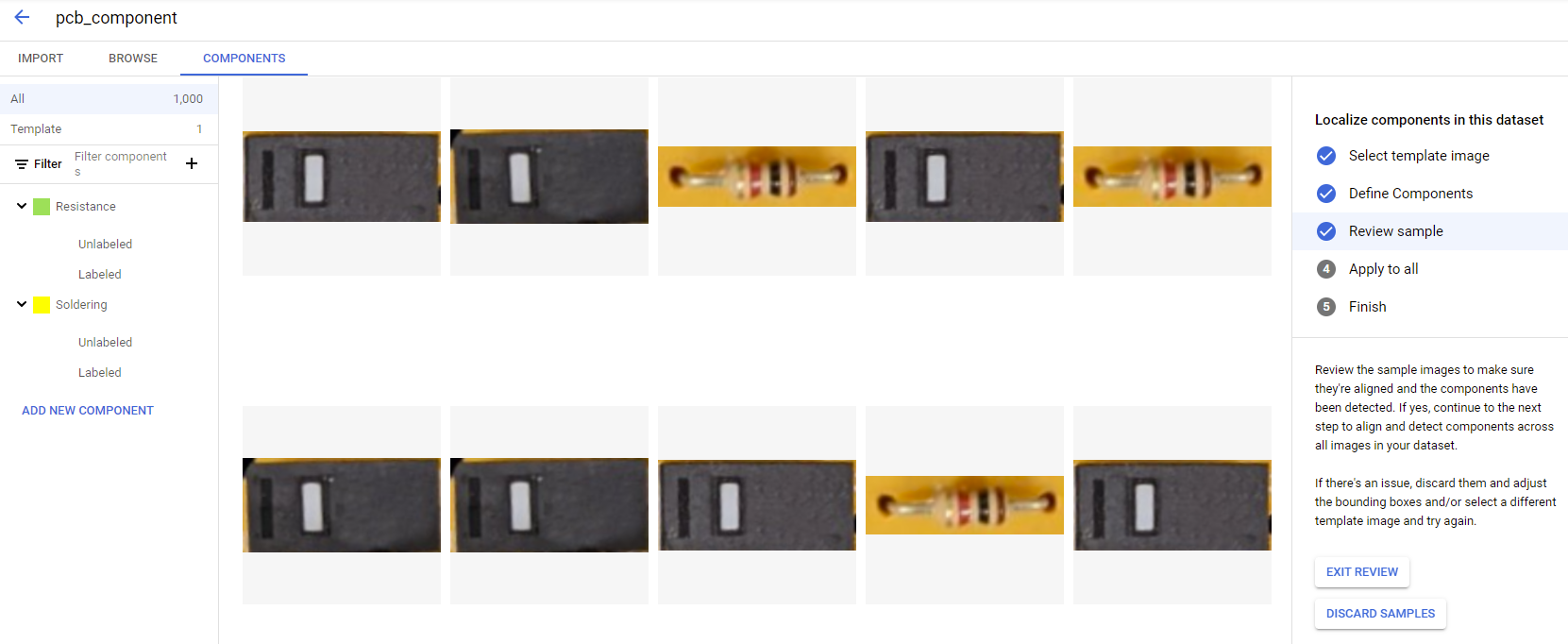
When the alignment process is complete, the candidate components are identified and displayed in the user interface. You will now review the output from the component detection and alignment step.
- Click the Next button to review the samples. A detailed view of the detected and cropped components region images will be displayed, all the Resistance component regions from all images have been detected and cropped.
If you are satisfied with the preview results of detected and cropped component regions, you can move to the next steps.
- Click the Apply to all status icon on the right side of the user interface panel, and then click the Apply button to formally apply the detection and cropping processes to all images. This will trigger another long running task and the Apply to all task status icon on the right side of the user interface panel indicates that the process is running.
Note: The Apply to all task will take about 15-20 minutes to complete. You do not need to wait for this step to finish.
Once the Apply to all task is completed, the Visual Inspection AI user interface will move to the Finish stage. This indicates that Visual Inspection is ready to use the detected and cropped component region images to train Visual Inspection AI Anomaly Detection models.
You have now completed the steps required to prepare for final model training. The training process will also take some time, well over an hour for this demo dataset. For this reason the rest of this lab provides an overview of the remaining steps involved in evaluating and refining a model and creating the solution artifact that can then be used to analyze images. In the follow up lab to this one, Deploying and Testing a Visual Inspection AI Component Anomaly Detection Solution, you learn how to deploy and use this solution artifact to analyze images.
If you were training your own model you would click the button to start training at this point, but you should not do that for this lab.
Note: The remaining sections of this lab are for information only, they are not steps that you should carry out in this lab session.
Overview 1. Training and refining an anomaly detection model
This section provides an overview of the procedures involved in training the component-based Anomaly Detection model. The cropped component images under each defined component initially do not have the ground-truth labels associated with them, however the Anomaly Detection model training in Visual Inspection AI allows you to kick off model training immediately without the need to provide any labels to the cropped component images. You can add the labels later and retrain the model to improve its accuracy.
The detailed detected and cropped view of each component can be viewed in the Components tab, under the component label Resistance.
To start the Anomaly Detection model training for the Resistance component, the Start Training option becomes available once component detection and alignment has completed. You might have to refresh your browser before the Start Training button appears. This button will disappear when training is being carried out and reappears again once it is complete.
Once the model training is started, the Train model task status icon is shown on the right side of the Visual Inspection user interface panel, indicating whether the training task is still in progress.
Note: For the demo dataset this first round of training your model would take about 50-60 minutes to complete.
Once model training has completed the Start Training button will be available again on the right panel, indicating that you can start a new round of training at any time.
Once a model has been trained the Go to evaluation review page button is also available on the right hand panel, allowing you to quickly navigate to the model evaluation page, which will be explored in more detail in the next section.
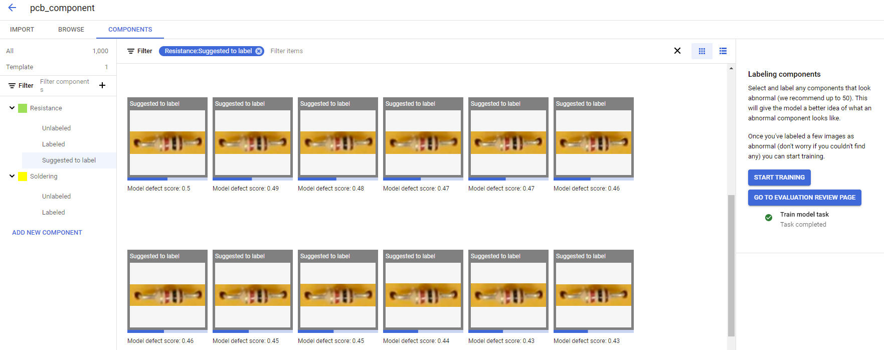
Clicking Suggested to label under Resistance switches to component images used during training that Visual Inspection AI has identified as the most useful for manual labeling.
For each of the component images, there will be a Model defect score associated with it. This score indicates how likely the trained model believes that this component image is defective. The higher the score, the more defective the model believes the component image to be. The value range of the Model defect score is from zero to one.
The images surrounded by the Suggested to label boxes are the images that the Visual Inspection AI system believes are most likely to need attention and verification, that is human labeling. If you follow these Suggested to label images, and verify them as either NORMAL or ABNORMAL, the human labeling information you provide on these images allows the Visual Inspection AI system to train a better Anomaly Detection model for the labeled component in subsequent rounds of Anomaly Detection model training.
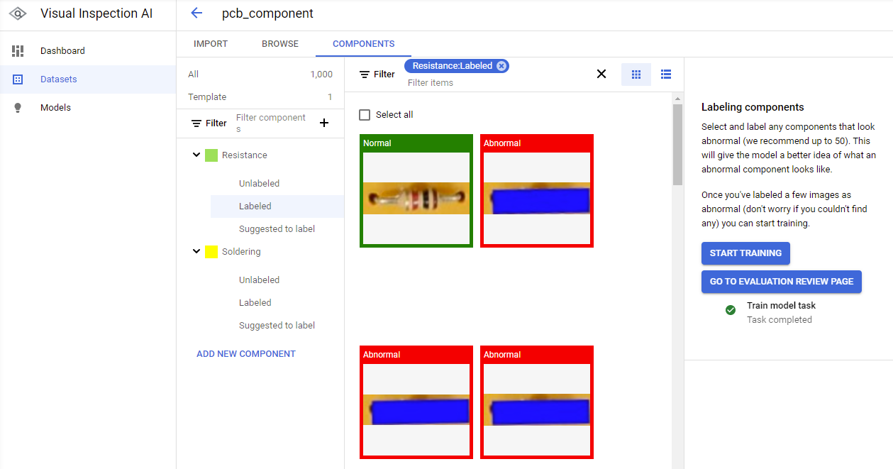
Some of the images in the demo dataset are deliberately masked to trigger defect detection using a blue rectangular mask and are used in this demo to make it easy to identify abnormal components. Labeling normal and abnormal components manually following a round of training helps to improve the accuracy of the model.
The images on the first page of Selected to label that contain a blue rectangle masking the resistor can be labeled as ABNORMAL by clicking the Label as abnormal option that appears in the pop-up above the images. These abnormal images are then highlighted in red.
Any remaining unassigned images on the first page of the Selected to label can then be labeled as NORMAL by clicking the Label as normal option that appears in the pop-up above the images. These normal images are then highlighted in green.
There are also two tabs, Unlabeled and Labeled, on the left panel that allow you to easily navigate through all the component images that you have already labeled under the Labeled tab, and the images you have not labeled yet under the Unlabeled tab.
Once NORMAL or ABNORMAL labels have been selected you can trigger a new round of Anomaly Detection model training to use these manually labeled components to improve the model.
Clicking on the Start Training button on the right side of the Visual Inspection AI user interface panel, will start another round of training.
Note: For the demo dataset this second round of training your model would take about 50-60 minutes to complete.
Once the component detection model is fully trained, inspecting the model's quality as well as exporting your trained Assembly Inspection solution artifact in the format of a docker image can be done through the Model page. The solution artifact Docker image can then be used to run batch predictions in the Cloud or you run the Docker container in an on-premises configuration.
Overview 2. Evaluating a trained Assembly Inspection model
This section demonstrates how to access and interpret the model evaluation user interface for a trained model.
Once the component's Anomaly Detection model has been trained, the trained model's performance can be checked from the Model page. There are two ways to navigate to the model evaluation page.
In the Anomaly Detection training page of the Resistance component, once model training is completed, there will be a Go to evaluation review page link showing up on the right panel as shown below:
The Model page icon on the left panel as shown below can be used to navigate to the model evaluation page:
Expanding the Dataset shows individually trained component Anomaly Detection models, in this case the model is Resistance.
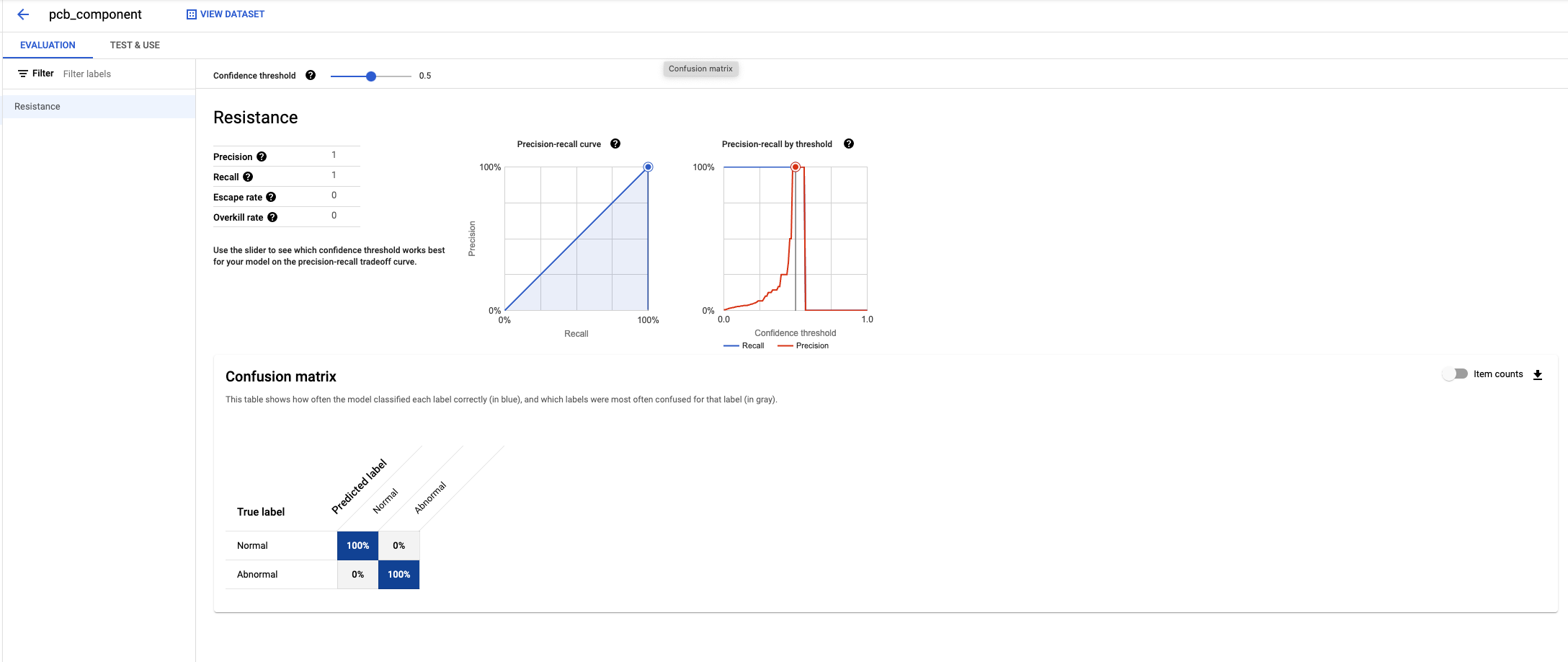
Clicking on the Resistance model, shows the detailed model evaluation page and results. The model evaluation detailed user interface page shows the Precision and Recall model evaluation metrics for the trained components Anomaly Detection models.
In the Visual Inspection AI Evaluation page, Positive data refers to images classified as defective, and Negative data refers to images classified as non-defective. This means:
True Positive (TP) is a defective image being correctly classified as defective.
False Positive (FP) is a non-defective image being wrongly classified as defective.
True Negative (TN) is a non-defective image being correctly classified as non-defective.
False Negative (FN) is a defective image being wrongly classified as non-defective.
The model evaluation metrics Precision and Recall are mathematically defined as follows:
Precision: TP / (TP + FP)
Recall: TP / (TP + FN)
The model evaluation page allows to modify the confidence threshold to evaluate the model using the Confidence threshold slider at the top of the page.
The page shows the confusion matrix calculated based on the component images ground-truth labels NORMAL and ABNORMAL that were labelled when refining the model. The confusion matrix allows to assess the model’s prediction output based on the selected confidence threshold to see how many false positives and false negatives are obtained at different confidence thresholds. Toggling the Item counts icon shows individual image count instead of the percentage numbers.
Overview 3. Creating a trained Component Assembly Detection solution artifact
This section provides an overview of the process of creating a trained Component Assembly Detection solution artifact.
After evaluating the results of the trained model, a trained solution artifact can be created in a docker format, and exported to a Container Registry location.
Note: Each component should be trained for anomaly detection prior to creating a Visual Inspection AI solution artifact.
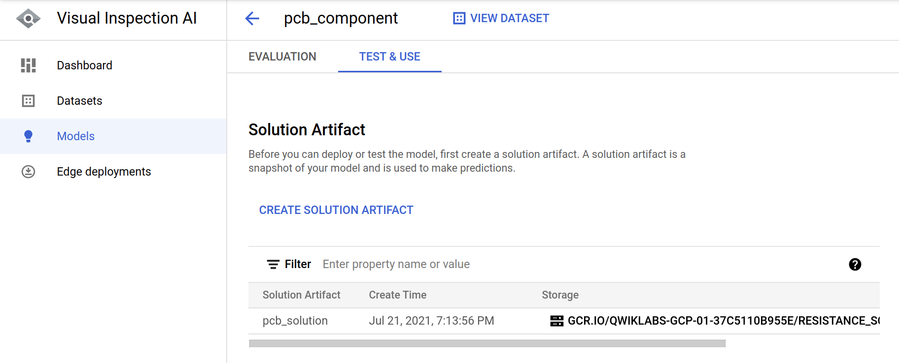
In the Test & Use tab on the Models page for the Resistance model, clicking Create Solution Artifact creates an Assembly Inspection solution artifact for a trained model.
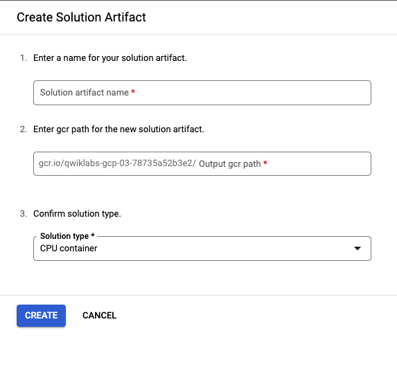
When creating the solution artifact you must specify the Solution artifact name, Cloud Source Repository Output gcr path, and the Solution type.
Note: You can select either a GPU or CPU container here. A GPU container can only be deployed to a container platform that supports the appropriate type of GPU. For the purposes of the next lab you can only test a CPU container so CPU is selected here.
Clicking Create triggers the solution artifact container image creation process.
It usually takes a couple of minutes to create the solution artifact.
At this stage the solution artifact is now ready and can be tested in the UI. This will allow you to check out the quality of the trained solution immediately using test images.
Overview 4. Performing batch predictions using an Assembly Inspection solution artifact
This section provides an overview of how to make batch predictions using the Assembly Inspection solution artifact created in the previous section.
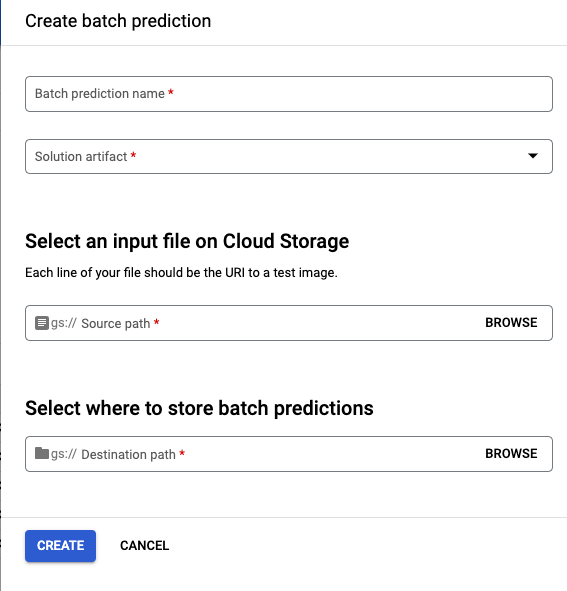
On Test & Use tab in the Models page, clicking on Create Batch Prediction starts a cloud batch prediction job using your solution container.
The following details are given to start a batch processing task:
| Field | Value |
| Batch prediction name | A name for this batch prediction test |
| Solution artifact | The ID of the Solution Artifact |
| gs:// Source Path | The path to a CSV file in a Cloud Storage bucket containing the image names. |
| Destination path | The path in the Cloud Storage bucket, where the JSON output file should be stored. |
Clicking Create starts the batch processing task.
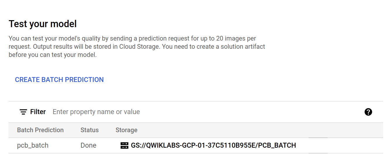
Clicking on the Storage link of the completed batch prediction job shows the batch prediction results and details.
The batch prediction data is contained in the JSON output file stored in the Cloud Storage bucket. An example of the output is shown below. You can see the data for each of the annotated components that have been detected as well as information about the source image.
{
    "annotationsGroups": [{
        "annotationSet": {
            "createTime": "2021-07-14T11:21:50.899029Z",
            "displayName": "Aligned Components",
            "name": "projects/574980676006/locations/us-central1/datasets/3804178290709626880/annotationSets/2092388219843772416",
            "polygon": {},
            "updateTime": "2021-07-14T11:50:25.404367Z"
        },
        "annotations": [{
            "annotationSetId": "2092388219843772416",
            "annotationSpecId": "2117339437212893184",
            "name": "localAnnotations/1000000",
            "polygon": {
                "normalizedBoundingPoly": {
                    "normalizedVertices": [{
                        "x": 0.50721323,
                        "y": 0.56952035
                    }, {
                        "x": 0.61584163,
                        "y": 0.58288085
                    }, {
                        "x": 0.61100781,
                        "y": 0.6221832
                    }, {
                        "x": 0.50237942,
                        "y": 0.6088227
                    }]
                }
            },
            "source": {
                "sourceModel": "projects/574980676006/locations/us-central1/solutions/3888084222048468992/modules/4022207048451096576/models/755901049956466688",
                "type": "MACHINE_PRODUCED"
            }
        }, {
            "annotationSetId": "2092388219843772416",
            "annotationSpecId": "2117339437212893184",
            "name": "localAnnotations/1000001",
            "polygon": {
                "normalizedBoundingPoly": {
                    "normalizedVertices": [{
                        "x": 0.61049843,
                        "y": 0.4533464
                    }, {
                        "x": 0.64012426,
                        "y": 0.45699003
                    }, {
                        "x": 0.62812692,
                        "y": 0.55453622
                    }, {
                        "x": 0.59850109,
                        "y": 0.55089259
                    }]
                }
            },
            "source": {
                "sourceModel": "projects/574980676006/locations/us-central11/solutions/3888084222048468992/modules/4022207048451096576/models/755901049956466688",
                "type": "MACHINE_PRODUCED"
            }
        }]
    }, {
        "annotationSet": {
            "classificationLabel": {},
            "createTime": "2021-07-14T11:50:25.386576Z",
            "displayName": "Output",
            "name": "projects/574980676006/locations/us-central1/datasets/3804178290709626880/annotationSets/6562210850008989696",
            "updateTime": "2021-07-14T11:50:25.666724Z"
        },
        "annotations": [{
            "annotationSetId": "6562210850008989696",
            "annotationSpecId": "332506609890623488",
            "classificationLabel": {
                "confidenceScore": 0.11153886
            },
            "name": "localAnnotations/0",
            "parentAnnotationId": "localAnnotations/1000000",
            "source": {
                "sourceModel": "projects/574980676006/locations/us-central1/solutions/3888084222048468992/modules/2553189144998182912/models/8294926826174676992",
                "type": "MACHINE_PRODUCED"
            }
        }, {
            "annotationSetId": "6562210850008989696",
            "annotationSpecId": "332506609890623488",
            "classificationLabel": {
                "confidenceScore": 0.019765764
            },
            "name": "localAnnotations/1",
            "parentAnnotationId": "localAnnotations/1000001",
            "source": {
                "sourceModel": "projects/574980676006/locations/us-central1/solutions/3888084222048468992/modules/2553189144998182912/models/8294926826174676992",
                "type": "MACHINE_PRODUCED"
            }
        }]
    }, {
        "annotationSet": {
            "createTime": "2021-07-14T11:21:50.815073Z",
            "displayName": "Aligned Inspection Areas",
            "name": "projects/574980676006/locations/us-central1/datasets/3804178290709626880/annotationSets/6794146230818570240",
            "polygon": {},
            "updateTime": "2021-07-14T11:21:50.815073Z"
        },
        "annotations": [{
            "annotationSetId": "6794146230818570240",
            "annotationSpecId": "8217465132486230016",
            "labels": {
                "goog_vi_annotation_set_name": "8538446661494505472",
                "goog_vi_transform_source_annotation_id": "6793052495921807360"
            },
            "name": "localAnnotations/1000002",
            "polygon": {
                "normalizedBoundingPoly": {
                    "normalizedVertices": [{
                        "x": 0.32404947,
                        "y": 0.16284555
                    }, {
                        "x": 0.83100849,
                        "y": 0.22519726
                    }, {
                        "x": 0.77095616,
                        "y": 0.71346146
                    }, {
                        "x": 0.26399708,
                        "y": 0.65110981
                    }]
                }
            },
            "source": {
                "sourceModel": "projects/574980676006/locations/us-central1/solutions/3888084222048468992/modules/4022207048451096576/models/755901049956466688",
                "type": "MACHINE_PRODUCED"
            }
        }]
    }],
    "predictedImageUri": "gs://qwiklabs-gcp-00-612891cc3352/demo_pcb_images/image_105_cx45_cy-55_r3.png"
}
Solution of Lab

