Overview

BigQuery is Google's fully managed, NoOps, low cost analytics database. With BigQuery you can query terabytes and terabytes of data without managing infrastructure or needing a database administrator. BigQuery uses SQL and takes advantage of the pay-as-you-go model. BigQuery allows you to focus on analyzing data to find meaningful insights.

BigQuery ML allows data analysts to use their SQL knowledge to build machine learning models quickly right where their data already lives in BigQuery.

In BigQuery, there is a publicly available dataset for NCAA basketball games, teams, and players. The game data covers play-by-play and box scores back to 2009, as well as final scores back to 1996. Additional data about wins and losses goes back to the 1894-5 season in some teams' cases.

In this lab, you use BigQuery ML to prototype, train, evaluate, and predict the 'winners' and 'losers' between two NCAA basketball tournament teams.

What you'll do

In this lab, you will learn how to:

• Use BigQuery to access the public NCAA dataset

• Explore the NCAA dataset to gain familiarity with the schema and scope of the data available

• Prepare and transform the existing data into features and labels

• Split the dataset into training and evaluation subsets

• Use BigQuery ML to build a model based on the NCAA tournament dataset

• Use your newly created model to predict NCAA tournament winners for your bracket

Prerequisites

This is an intermediate level lab. Before taking it, you should have some experience with SQL and the language's keywords. Familiarity with BigQuery is also recommended. If you need to get up to speed in these areas, you should at a minimum take one of the following labs before attempting this one:

• Introduction to SQL for BigQuery and Cloud SQL

• BigQuery: Qwik Start - Console

Setup and requirements

Before you click the Start Lab button

Read these instructions. Labs are timed and you cannot pause them. The timer, which starts when you click Start Lab, shows how long Google Cloud resources will be made available to you.

This hands-on lab lets you do the lab activities yourself in a real cloud environment, not in a simulation or demo environment. It does so by giving you new, temporary credentials that you use to sign in and access Google Cloud for the duration of the lab.

To complete this lab, you need:

• Access to a standard internet browser (Chrome browser recommended).

Note: Use an Incognito or private browser window to run this lab. This prevents any conflicts between your personal account and the Student account, which may cause extra charges incurred to your personal account.

• Time to complete the lab---remember, once you start, you cannot pause a lab.

Note: If you already have your own personal Google Cloud account or project, do not use it for this lab to avoid extra charges to your account.

How to start your lab and sign in to the Google Cloud console

1. Click the Start Lab button. If you need to pay for the lab, a pop-up opens for you to select your payment method. On the left is the Lab Details panel with the following:

   • The Open Google Cloud console button

   • Time remaining

   • The temporary credentials that you must use for this lab

   • Other information, if needed, to step through this lab

2. Click Open Google Cloud console (or right-click and select Open Link in Incognito Window if you are running the Chrome browser).

   The lab spins up resources, and then opens another tab that shows the Sign in page.

   Tip: Arrange the tabs in separate windows, side-by-side.

   Note: If you see the Choose an account dialog, click Use Another Account.

3. If necessary, copy the Username below and paste it into the Sign in dialog.

    student-04-bfede1434629@qwiklabs.net
   

   You can also find the Username in the Lab Details panel.

4. Click Next.

5. Copy the Password below and paste it into the Welcome dialog.

    EA654l3afWkG
   

   You can also find the Password in the Lab Details panel.

6. Click Next.

   Important: You must use the credentials the lab provides you. Do not use your Google Cloud account credentials.

   Note: Using your own Google Cloud account for this lab may incur extra charges.

7. Click through the subsequent pages:

   • Accept the terms and conditions.

   • Do not add recovery options or two-factor authentication (because this is a temporary account).

   • Do not sign up for free trials.

After a few moments, the Google Cloud console opens in this tab.

Note: To view a menu with a list of Google Cloud products and services, click the Navigation menu at the top-left.

Open the BigQuery console

1. In the Google Cloud Console, select Navigation menu > BigQuery.

The Welcome to BigQuery in the Cloud Console message box opens. This message box provides a link to the quickstart guide and the release notes.

2. Click Done.

The BigQuery console opens.

Task 1. Open the BigQuery console

1. From the Cloud Console, open the Navigation menu and select BigQuery.

2. Click DONE to take yourself to the beta UI. Make sure that your Project ID is set in Explorer tab, which should resemble the following:

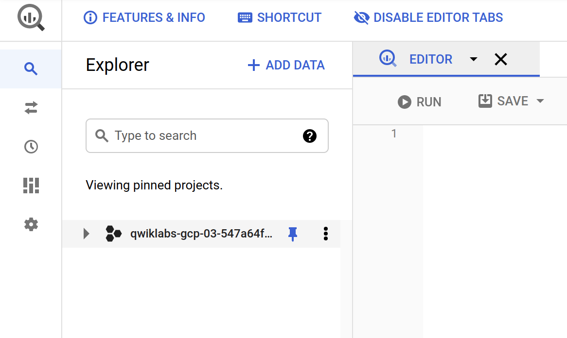
If you click Expand node arrow next to your project, you won't see any databases or tables there. This is because you haven't added any to your project yet.

Luckily, there are tons of open, public datasets available in BigQuery for you to work with. You will now learn more about the NCAA dataset and then figure out how to add the dataset to your BigQuery project.

Task 2. NCAA March Madness

The National Collegiate Athletic Association (NCAA) hosts two major college basketball tournaments every year in the United States for men's and women's collegiate basketball. For the NCAA Men's tournament in March, 68 teams enter single-elimination games and one team exits as the overall winner of March Madness.

The NCAA offers a public dataset that contains the statistics for men's and women's basketball games and players in for the season and the final tournaments. The game data covers play-by-play and box scores back to 2009, as well as final scores back to 1996. Additional data about wins and losses goes back to the 1894-5 season in some teams' cases.

• Be sure to check out the Google Cloud Marketing Ad campaign for predicting live insights to learn a little bit more about this dataset and what's been done with it and stay up to date with this year's tournament at Google Cloud March Madness Insights.

Task 3. Find the NCAA public dataset in BigQuery

1. Make sure that you are still in the BigQuery Console for this step. In the Explorer tab, click the + ADD button then select Public datasets.

2. In the search bar, type in NCAA Basketball and hit enter. One result will pop up—select it and then click VIEW DATASET:

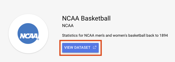
This will open a new BigQuery tab with the dataset loaded. You can continue working in this tab, or close it and refresh your BigQuery Console in the other tab to reveal your public dataset.

Note: If you are unable to see the ncaa_basketball then click on + ADD > Star a project by name. Enter bigquery-public-data as the project name and then click STAR.

3. Expand bigquery-public-data > ncaa_basketball dataset to reveal its tables:

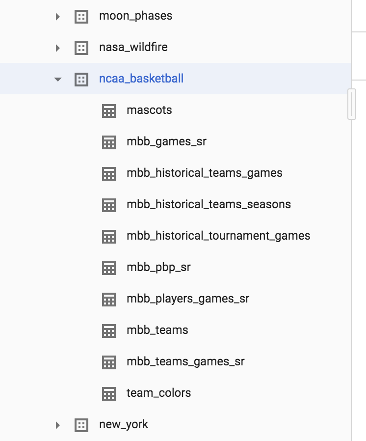
You should see 10 tables in the dataset.

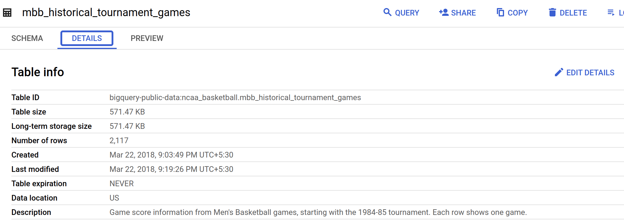
4. Click on the mbb_historical_tournament_games and then click PREVIEW to see sample rows of data.

5. Then click DETAILS to get metadata about the table.

Your page should resemble the following:

Task 4. Write a query to determine available seasons and games

You will now write a simple SQL query to determine how many seasons and games are available to explore in our mbb_historical_tournament_games table.

1. In query EDITOR, which is located above the table details section, copy and paste the following into that field:

SELECT
  season,
  COUNT(*) as games_per_tournament
  FROM
 `bigquery-public-data.ncaa_basketball.mbb_historical_tournament_games`
 GROUP BY season
 ORDER BY season # default is Ascending (low to high)

2. Click RUN. Soon after, you should receive a similar output:

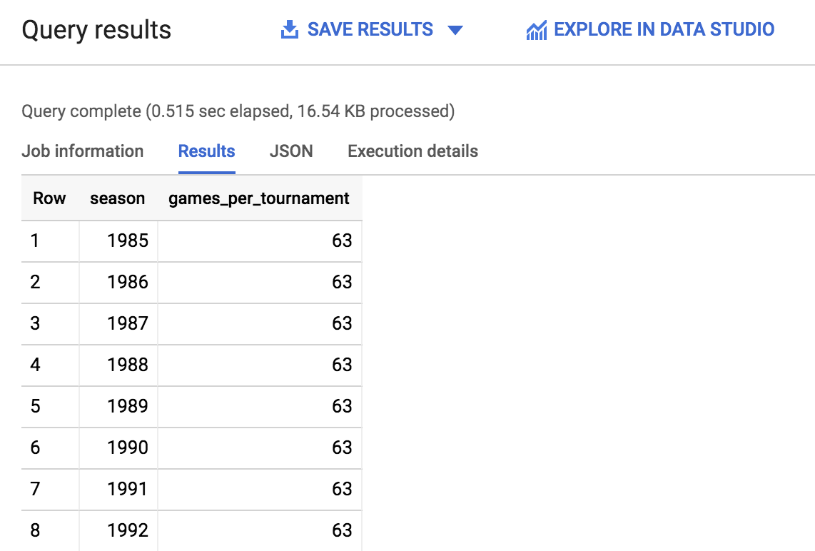
3. Scroll through the output and take note of the amount of seasons and the games played per season—you will use that information to answer the following questions. Additionally, you can quickly see how many rows were returned by looking in the lower right near the pagination arrows.

Click Check my progress to verify the objective.

Write a query to determine available seasons and games

Check my progress

Test your understanding

The following multiple choice questions are used to reinforce your understanding of the concepts covered so far. Answer them to the best of your abilities.

How many NCAA Men's Basketball tournament seasons (i.e. 1985, 1986..) are available for us to explore?67637033

Submit

How far back in time does the data in the NCAA Men's Basketball tournament data go for this table?2019198619852017

Submit

Task 5. Understand machine learning features and labels

The end goal of this lab is to predict the winner of a given NCAA Men's basketball match-up using past knowledge of historical games. In machine learning, each column of data that will help us determine the outcome (win or loss for a tournament game) is called a feature.

The column of data that you are trying to predict is called the label. Machine learning models "learn" the association between features to predict the outcome of a label.

Examples of features for your historical dataset could be:

• Season

• Team name

• Opponent team name

• Team seed (ranking)

• Opponent team seed

The label you will be trying to predict for future games will be the game outcome — whether or not a team wins or loses.

Test your understanding

The following multiple choice questions are used to reinforce your understanding of the concepts covered so far. Answer them to the best of your abilities.

For our historical training dataset, we know the correct answer for our labels (i.e. we know who won or lost)TrueFalse

Submit

For future predictions, we know the correct answer for our labels at the time of prediction.TrueFalse

Submit

Task 6. Create a labeled machine learning dataset

Building a machine learning model requires a lot of high-quality training data. Fortunately, our NCAA dataset is robust enough where we can rely upon it to build an effective model.

1. Return to the BigQuery Console—you should have left off on the result of the query you ran.

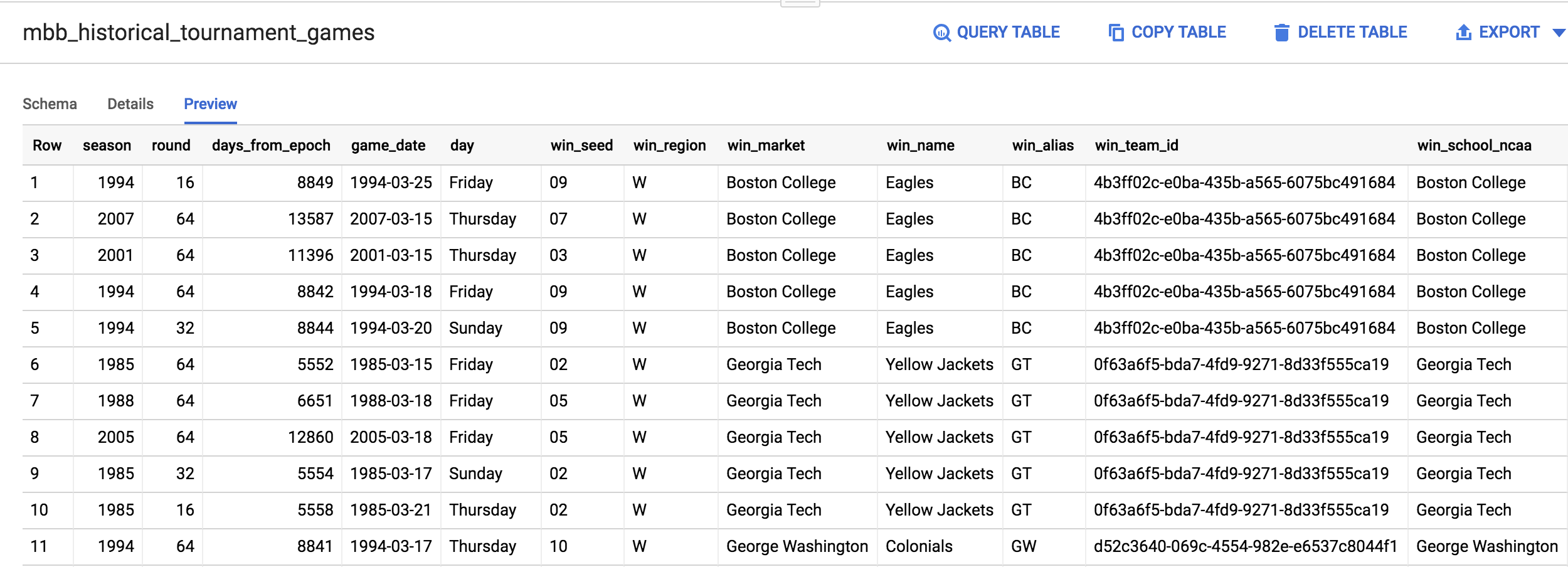
2. From the left-hand menu, open the mbb_historical_tournament_games table by clicking on the table name. Then once it loads, click PREVIEW. Your page should resemble the following:

Test your understanding

The following multiple choice questions are used to reinforce your understanding of the concepts covered so far. Answer them to the best of your abilities.

Our labeled column for the outcome of the game already exists as a column in our dataset (i.e. a column that says WIN or LOSS)TrueFalse

Submit

For each specific basketball game, the dataset has one row for the winner and one row for the loser.TrueFalse

Submit

3. After inspecting the dataset, you'll notice that one row in the dataset has columns for both win_market and lose_market. You need to break the single game record into a record for each team so you can label each row as a "winner" or "loser".

4. In the query EDITOR, copy and paste the following query and then click RUN:

# create a row for the winning team
SELECT
  # features
  season, # ex: 2015 season has March 2016 tournament games
  round, # sweet 16
  days_from_epoch, # how old is the game
  game_date,
  day, # Friday

  'win' AS label, # our label

  win_seed AS seed, # ranking
  win_market AS market,
  win_name AS name,
  win_alias AS alias,
  win_school_ncaa AS school_ncaa,
  # win_pts AS points,

  lose_seed AS opponent_seed, # ranking
  lose_market AS opponent_market,
  lose_name AS opponent_name,
  lose_alias AS opponent_alias,
  lose_school_ncaa AS opponent_school_ncaa
  # lose_pts AS opponent_points

FROM `bigquery-public-data.ncaa_basketball.mbb_historical_tournament_games`

UNION ALL

# create a separate row for the losing team
SELECT
# features
  season,
  round,
  days_from_epoch,
  game_date,
  day,

  'loss' AS label, # our label

  lose_seed AS seed, # ranking
  lose_market AS market,
  lose_name AS name,
  lose_alias AS alias,
  lose_school_ncaa AS school_ncaa,
  # lose_pts AS points,

  win_seed AS opponent_seed, # ranking
  win_market AS opponent_market,
  win_name AS opponent_name,
  win_alias AS opponent_alias,
  win_school_ncaa AS opponent_school_ncaa
  # win_pts AS opponent_points

FROM
`bigquery-public-data.ncaa_basketball.mbb_historical_tournament_games`

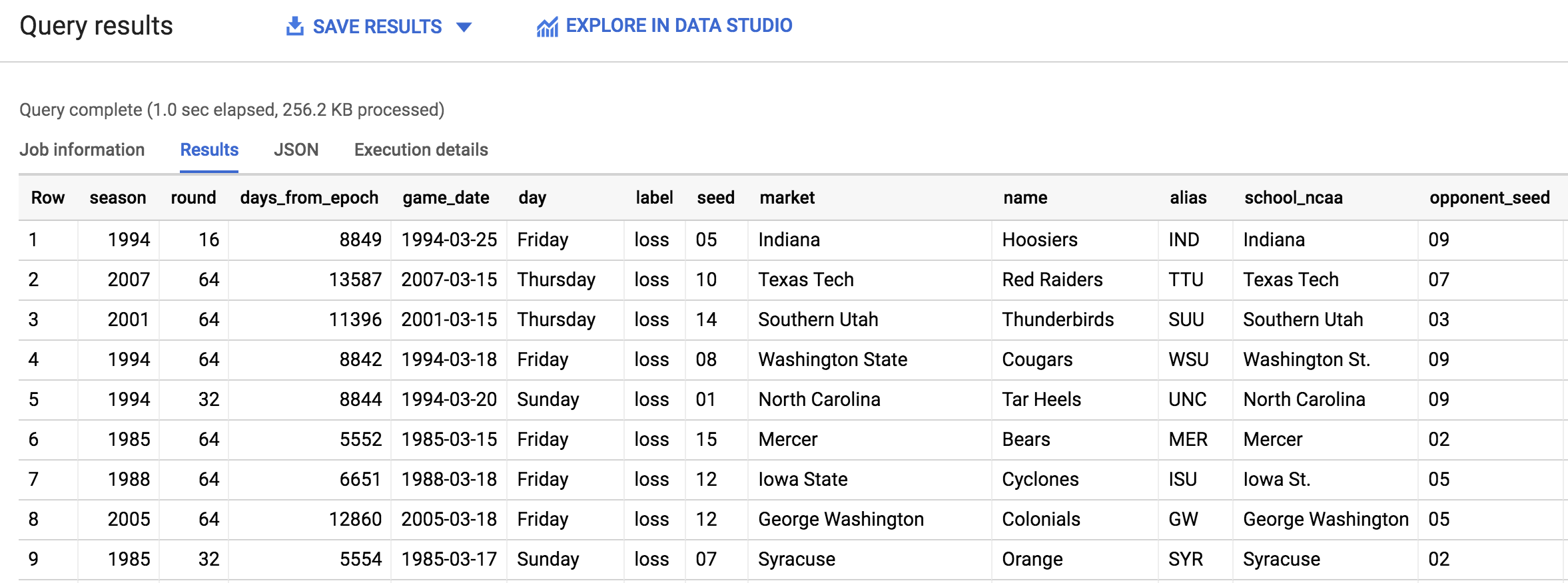
You should receive the following output:

Click Check my progress to verify the objective.

Create a labeled machine learning dataset

Check my progress

Now that you know what features are available from the result, answer the following question to reinforce your understanding of the dataset.

Why should we NOT use the points scored (win_pts or lose_pts) as a feature in our training dataset if we have the data available?This feature is numerical and cannot be used in a classification model.This feature is only available at the END of the game and for future games we are making predictions before a game begins.This feature is only populated for recent games and should not be used.

Submit

Task 7. Create a machine learning model to predict the winner based on seed and team name

Now that we have explored our data, it's time to train a machine learning model.

• Using your best judgment, answer the question below to orient yourself with this section.

What type of machine learning model should we build knowing our goal is to predict game outcome (either win or lose)We should build a forecasting model to predict how many points a team will score in a particular game.We should build a classification model to predict whether a team will win or lose a particular game.

Submit

Choosing a model type

For this particular problem, you will be building a classification model. Since we have two classes, win or lose, it's also called a binary classification model. A team can either win or lose a match.

If you wanted to, after the lab, you could forecast the total number of points a team will score using a forecasting model but that isn't going to be our focus here.

An easy way to tell if you're forecasting or classifying is to look at the type of label (column) of data you are predicting:

• If it's a numeric column (like units sold or points in a game), you're doing forecasting

• If it's a string value you're doing classification (this row is either this in class or this other class), and

• If you have more than two classes (like win, lose, or tie) you are doing multi-class classification

Our classification model will be doing machine learning with a widely used statistical model called Logistic Regression.

We need a model that generates a probability for each possible discrete label value, which in our case is either a 'win' or a 'loss'. Logistic regression is a good model type to start with for this purpose. The good news for you is that the ML model will do all the math and optimization for you during model training -- it's what computers are really good at!

Note: There are many other machine learning models that vary in complexity to perform classification tasks. One commonly used at Google is Deep Learning with Neural Networks.

Creating a machine learning model with BigQuery ML

To create our classification model in BigQuery we simply need to write the SQL statement CREATE MODEL and provide a few options.

But, before we can create the model, we need a place in our project to store it first.

1. In the Explorer tab, click on the View actions icon next to your Project ID and select Create dataset.

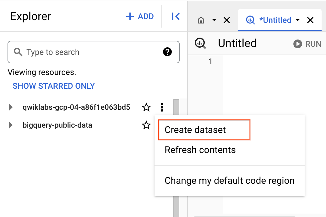
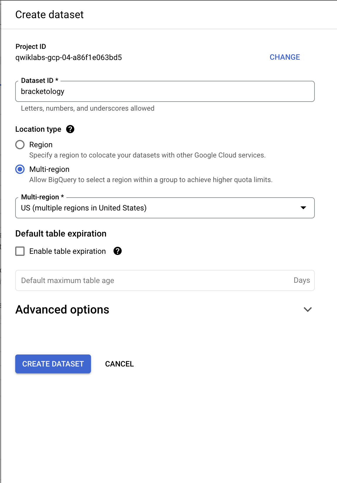
2. This will open a Create dataset dialog. Set your Dataset ID to bracketology and click CREATE DATASET.

3. Now run the following command in the query EDITOR

CREATE OR REPLACE MODEL
  `bracketology.ncaa_model`
OPTIONS
  ( model_type='logistic_reg') AS

# create a row for the winning team
SELECT
  # features
  season,

  'win' AS label, # our label

  win_seed AS seed, # ranking
  win_school_ncaa AS school_ncaa,

  lose_seed AS opponent_seed, # ranking
  lose_school_ncaa AS opponent_school_ncaa

FROM `bigquery-public-data.ncaa_basketball.mbb_historical_tournament_games`
WHERE season <= 2017

UNION ALL

# create a separate row for the losing team
SELECT
# features
  season,

  'loss' AS label, # our label
  lose_seed AS seed, # ranking
  lose_school_ncaa AS school_ncaa,

  win_seed AS opponent_seed, # ranking
  win_school_ncaa AS opponent_school_ncaa

FROM
`bigquery-public-data.ncaa_basketball.mbb_historical_tournament_games`

# now we split our dataset with a WHERE clause so we can train on a subset of data and then evaluate and test the model's performance against a reserved subset so the model doesn't memorize or overfit to the training data.

# tournament season information from 1985 - 2017
# here we'll train on 1985 - 2017 and predict for 2018
WHERE season <= 2017

In our code you'll notice that creating the model is just a few lines of SQL. One of the most important options is choosing the model type logistic_reg for our classification task.

Note: Refer to the BigQuery ML documentation guide for a list of all available model options and settings. In our case we already have a field named "label" so we avoid having to specify our label column by using the model option: input_label_cols.

It will take between 3 and 5 minutes to train the model. You should receive the following output when the job is finished:

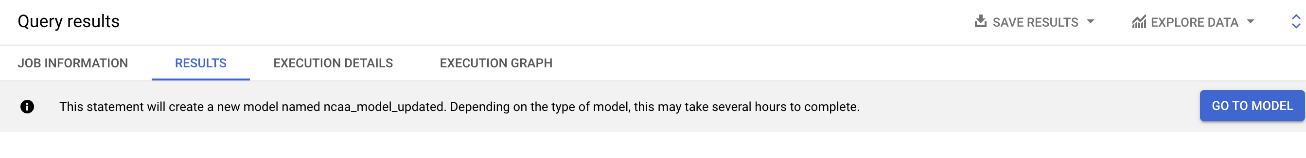
4. Click the Go to Model button on the right-hand side of the console.

Click Check my progress to verify the objective.

Create a machine learning model

Check my progress

View model training details

• Now that you are in the model details, scroll down to the Training options section and see the actual iterations the model performed to train.

If you're experienced with machine learning, note that you can customize all of these hyperparameters (options set before the model runs) by defining their value in the OPTIONS statement.

If you're new to machine learning, BigQuery ML will set smart default values for any options not set.

Refer to the BigQuery ML model options list to learn more.

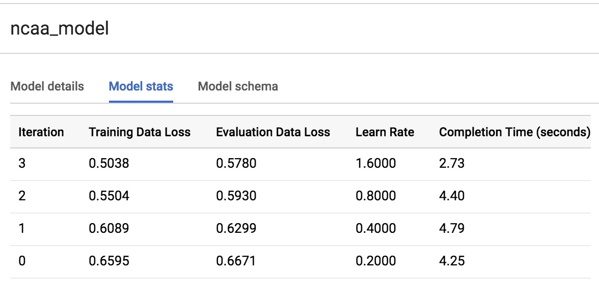
View model training stats

Machine learning models "learn" the association between known features and unknown labels. As you might intuitively guess, some features like "ranking seed" or "school name" may help determine a win or loss more than other data columns (features) like the day of the week the game is played.

Machine learning models start the training process with no such intuition and will generally randomize the weighting of each feature.

During the training process, the model will optimize a path to it's best possible weighting of each feature. With each run it is trying to minimize Training Data Loss and Evaluation Data Loss.

Should you ever find that the final loss for evaluation is much higher than for training, your model is overfitting or memorizing your training data instead of learning generalizable relationships.

You can view how many training runs the model takes by clicking the TRAINING tab and selecting Table under View as option.

During our particular run, the model completed 3 training iterations in about 20 seconds. Yours will likely vary.

See what the model learned about our features

After training, you can see which features provided the most value to the model by inspecting the weights.

• Run the following command in the query EDITOR:

SELECT
  category,
  weight
FROM
  UNNEST((
    SELECT
      category_weights
    FROM
      ML.WEIGHTS(MODEL `bracketology.ncaa_model`)
    WHERE
      processed_input = 'seed')) # try other features like 'school_ncaa'
      ORDER BY weight DESC

Your output should resemble the following:

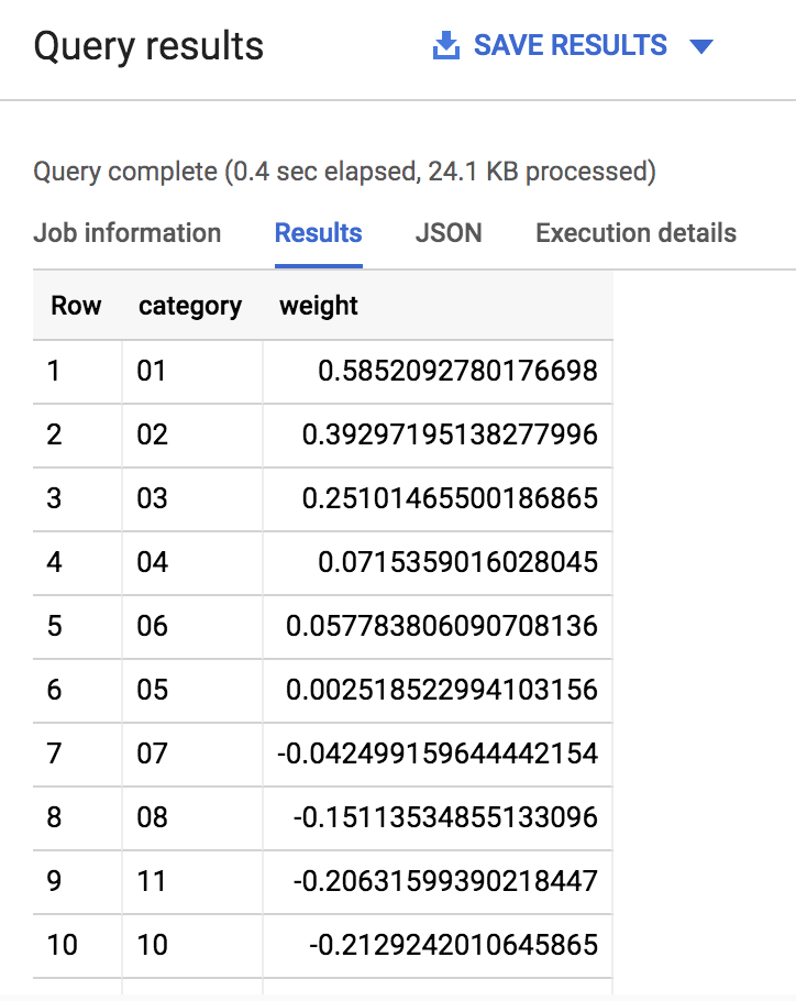
As you can see, if the seed of a team is very low (1,2,3) or very high (14,15,16) the model gives it a significant weight (max is 1.0) in determining the win loss outcome. Intuitively this makes sense as we expect very low seed teams to perform well in the tournament.

The real magic of machine learning is that we didn't create a ton of hardcoded IF THEN statements in SQL telling the model IF the seed is 1 THEN gives the team a 80% more chance of winning. Machine learning does away with hardcoded rules and logic and learns these relationships for itself. Check out the BQML syntax weights documentation to learn more.

Task 8. Evaluate model performance

To evaluate the model's performance you can run a simple ML.EVALUATE against a trained model.

• Run the following command in the query EDITOR:

SELECT
  *
FROM
  ML.EVALUATE(MODEL   `bracketology.ncaa_model`)

You should receive a similar output:

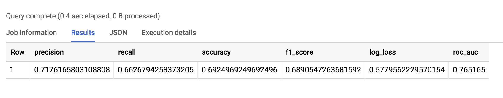
The value will be around 69% accurate. While it's better than a coin flip, there is room for improvement.

Note: For classification models, model accuracy isn't the only metric in the output you should care about.

Because you performed a logistic regression, you can evaluate your model performance against all of the following metrics (the closer to 1.0 the better):

• Precision: A metric for classification models. Precision identifies the frequency with which a model was correct when predicting the positive class.

• Recall: A metric for classification models that answers the following question: Out of all the possible positive labels, how many did the model correctly identify?

• Accuracy: Accuracy is the fraction of predictions that a classification model got right.

• f1_score: A measure of the accuracy of the model. The f1 score is the harmonic average of the precision and recall. An f1 score's best value is 1. The worst value is 0.

• log_loss: The loss function used in a logistic regression. This is the measure of how far the model's predictions are from the correct labels.

• roc_auc: The area under the ROC curve. This is the probability that a classifier is more confident that a randomly chosen positive example is actually positive than that a randomly chosen negative example is positive.

What do you think we could do to improve the model accuracy?Add back the total points scored in the tournament game to the training datasetOur data only looks at NCAA tournament data which is a small part of the entire basketball season. If we included data on the regular season games the model may learn additional insights about the teamsExperiment with adding more features from our initial dataset and re-training the model (feature engineering).

Submit

Task 9. Making predictions

Now that you trained a model on historical data up to and including the 2017 season (which was all the data you had), it's time to make predictions for the 2018 season. Your data science team has just provided you with the tournament results for the 2018 tournament in a separate table which you don't have in your original dataset.

Making predictions is as simple as calling ML.PREDICT on a trained model and passing through the dataset you want to predict on.

• Run the following command in the query EDITOR:

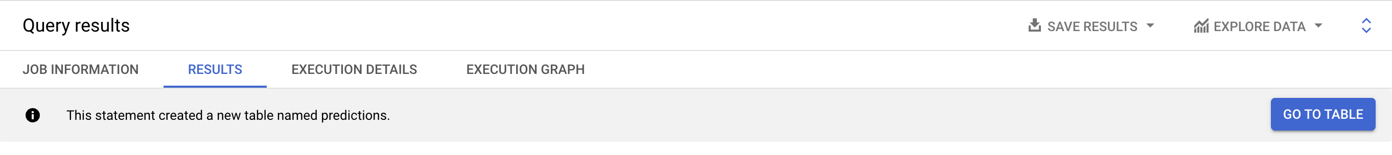
CREATE OR REPLACE TABLE `bracketology.predictions` AS (

SELECT * FROM ML.PREDICT(MODEL `bracketology.ncaa_model`,

# predicting for 2018 tournament games (2017 season)
(SELECT * FROM `data-to-insights.ncaa.2018_tournament_results`)
)
)

You should receive a similar output soon after:

Click Check my progress to verify the objective.

Evaluate model performance and create table

Check my progress

Why could we bring back the data columns for win_pts, lose_pts, game_date, and round in our prediction? Isn't that not allowed?The model is already trained. Adding these columns back during prediction-time provides additional context for the user but they do not get used as model features.You should not include these new columns in your prediction output.The model is already trained. Using these new data columns now will only increase the accuracy of the prediction.

Submit

Note: You're storing your predictions in a table so you can query for insights later without having to keep re-running the above query.

You will now see your original dataset plus the addition of three new columns:

• Predicted label

• Predicted label options

• Predicted label probability

Since you happen to know the results of the 2018 March Madness tournament, let's see how the model did with its predictions. (Tip: If you're predicting for this year's March Madness tournament, you would simply pass in a dataset with 2019 seeds and team names. Naturally, the label column will be empty as those games haven't been played yet -- that's what you're predicting!).

Task 10. How many did our model get right for the 2018 NCAA tournament?

• Run the following command in the query EDITOR:

SELECT * FROM `bracketology.predictions`
WHERE predicted_label <> label

You should receive a similar output:

Out of 134 predictions (67 March tournament games), our model got it wrong 38 times. 70% overall for the 2018 tournament matchup.

Task 11. Models can only take you so far...

There are many other factors and features that go into the close wins and amazing upsets of any March Madness tournament that a model would have a very hard time predicting.

Let's find biggest upset for the 2017 tournament according to the model. We'll look where the model predicts with 80%+ confidence and gets it WRONG.

1. Run the following command in the query EDITOR:

SELECT
  model.label AS predicted_label,
  model.prob AS confidence,

  predictions.label AS correct_label,

  game_date,
  round,

  seed,
  school_ncaa,
  points,

  opponent_seed,
  opponent_school_ncaa,
  opponent_points

FROM `bracketology.predictions` AS predictions,
UNNEST(predicted_label_probs) AS model

WHERE model.prob > .8 AND predicted_label <> predictions.label

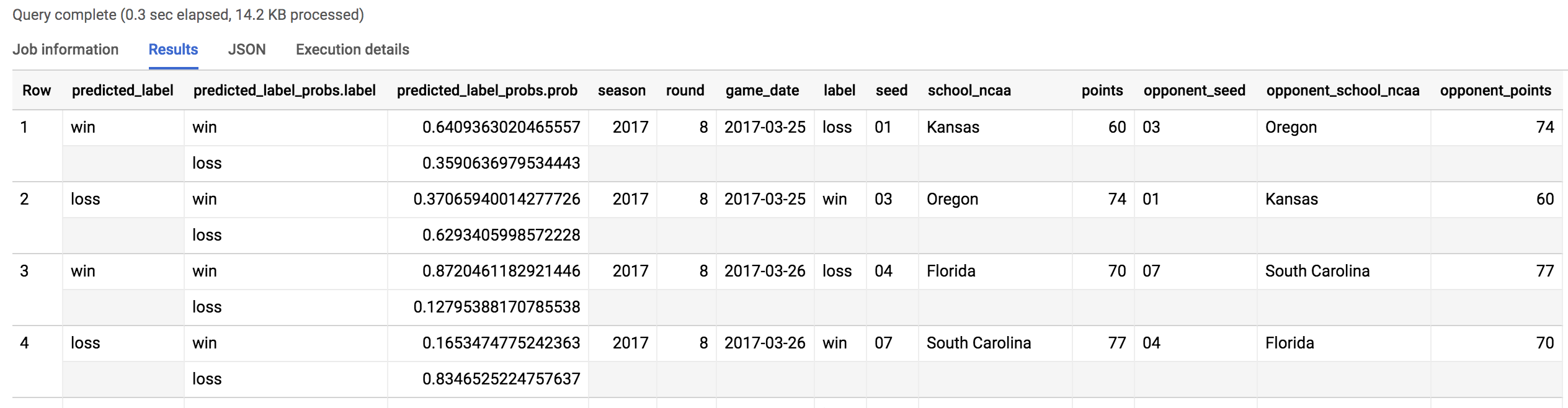
The outcome should look like this:

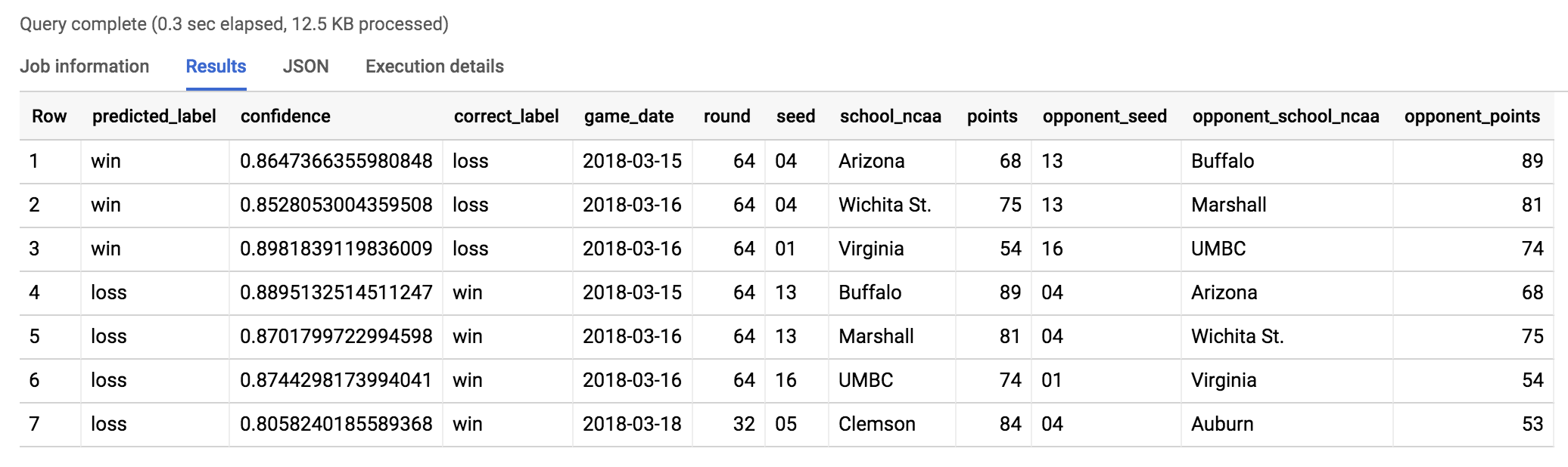
Prediction: The model predicts Seed 1 Virginia to beat Seed 16 UMBC with 87% confidence. Seems reasonable right?

Take a look at the '16-seed UMBC pulls off a miracle upset over 1-seed Virginia' video to see what actually happened!

Coach Odom (UMBC) after the game said, "Unbelievable — it’s really all you can say." Read more about it in the 2018 UMBC vs. Virginia men's basketball game article.

Recap

• You created a machine learning model to predict game outcome.

• You evaluated the performance and got to 69% accuracy using seed and team name as primary features

• You predicted 2018 tournament outcomes

• You analyzed the results for insights

Our next challenge will be to build a better model WITHOUT using seed and team name as features.

Task 12. Using skillful ML model features

In the second part of this lab you will be building a second ML model using newly provided and detailed features.

What is a shortcoming of our first model?The model heavily relied on team name as a feature. This punishes teams who had poor performance in previous years even if they have an all-star undefeated team this season.The model largely learned that lower seeded teams (1,2,3) would always beat higher seed teams (14,15,16).The training dataset was limited to team name and seed. It ignored other key features like the pace or scoring efficiency of each team.All of the above

Submit

Now that you're familiar with building ML models using BigQuery ML, your data science team has provided you with a new play-by-play dataset where they have created new team metrics for your model to learn from. These include:

• Scoring efficiency over time based on historical play-by-play analysis.

• Possession of the basketball over time.

Create a new ML dataset with these skillful features

• Run the following command in the query EDITOR:

# create training dataset:
# create a row for the winning team
CREATE OR REPLACE TABLE `bracketology.training_new_features` AS
WITH outcomes AS (
SELECT
  # features
  season, # 1994

  'win' AS label, # our label

  win_seed AS seed, # ranking # this time without seed even
  win_school_ncaa AS school_ncaa,

  lose_seed AS opponent_seed, # ranking
  lose_school_ncaa AS opponent_school_ncaa

FROM `bigquery-public-data.ncaa_basketball.mbb_historical_tournament_games` t
WHERE season >= 2014

UNION ALL

# create a separate row for the losing team
SELECT
# features
  season, # 1994

  'loss' AS label, # our label

  lose_seed AS seed, # ranking
  lose_school_ncaa AS school_ncaa,

  win_seed AS opponent_seed, # ranking
  win_school_ncaa AS opponent_school_ncaa

FROM
`bigquery-public-data.ncaa_basketball.mbb_historical_tournament_games` t
WHERE season >= 2014

UNION ALL

# add in 2018 tournament game results not part of the public dataset:
SELECT
  season,
  label,
  seed,
  school_ncaa,
  opponent_seed,
  opponent_school_ncaa
FROM
  `data-to-insights.ncaa.2018_tournament_results`

)

SELECT
o.season,
label,

# our team
  seed,
  school_ncaa,
  # new pace metrics (basketball possession)
  team.pace_rank,
  team.poss_40min,
  team.pace_rating,
  # new efficiency metrics (scoring over time)
  team.efficiency_rank,
  team.pts_100poss,
  team.efficiency_rating,

# opposing team
  opponent_seed,
  opponent_school_ncaa,
  # new pace metrics (basketball possession)
  opp.pace_rank AS opp_pace_rank,
  opp.poss_40min AS opp_poss_40min,
  opp.pace_rating AS opp_pace_rating,
  # new efficiency metrics (scoring over time)
  opp.efficiency_rank AS opp_efficiency_rank,
  opp.pts_100poss AS opp_pts_100poss,
  opp.efficiency_rating AS opp_efficiency_rating,

# a little feature engineering (take the difference in stats)

  # new pace metrics (basketball possession)
  opp.pace_rank - team.pace_rank AS pace_rank_diff,
  opp.poss_40min - team.poss_40min AS pace_stat_diff,
  opp.pace_rating - team.pace_rating AS pace_rating_diff,
  # new efficiency metrics (scoring over time)
  opp.efficiency_rank - team.efficiency_rank AS eff_rank_diff,
  opp.pts_100poss - team.pts_100poss AS eff_stat_diff,
  opp.efficiency_rating - team.efficiency_rating AS eff_rating_diff

FROM outcomes AS o
LEFT JOIN `data-to-insights.ncaa.feature_engineering` AS team
ON o.school_ncaa = team.team AND o.season = team.season
LEFT JOIN `data-to-insights.ncaa.feature_engineering` AS opp
ON o.opponent_school_ncaa = opp.team AND o.season = opp.season

You should receive a similar output soon after:

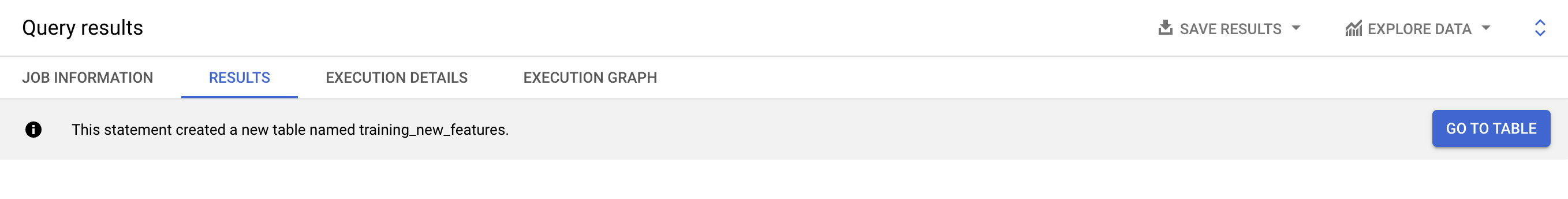
Click Check my progress to verify the objective.

Using skillful ML model features

Check my progress

Task 13. Preview the new features

• Click on the Go to table button on the right-hand side of the console. Then click on the Preview tab.

Your table should look similar to the following:

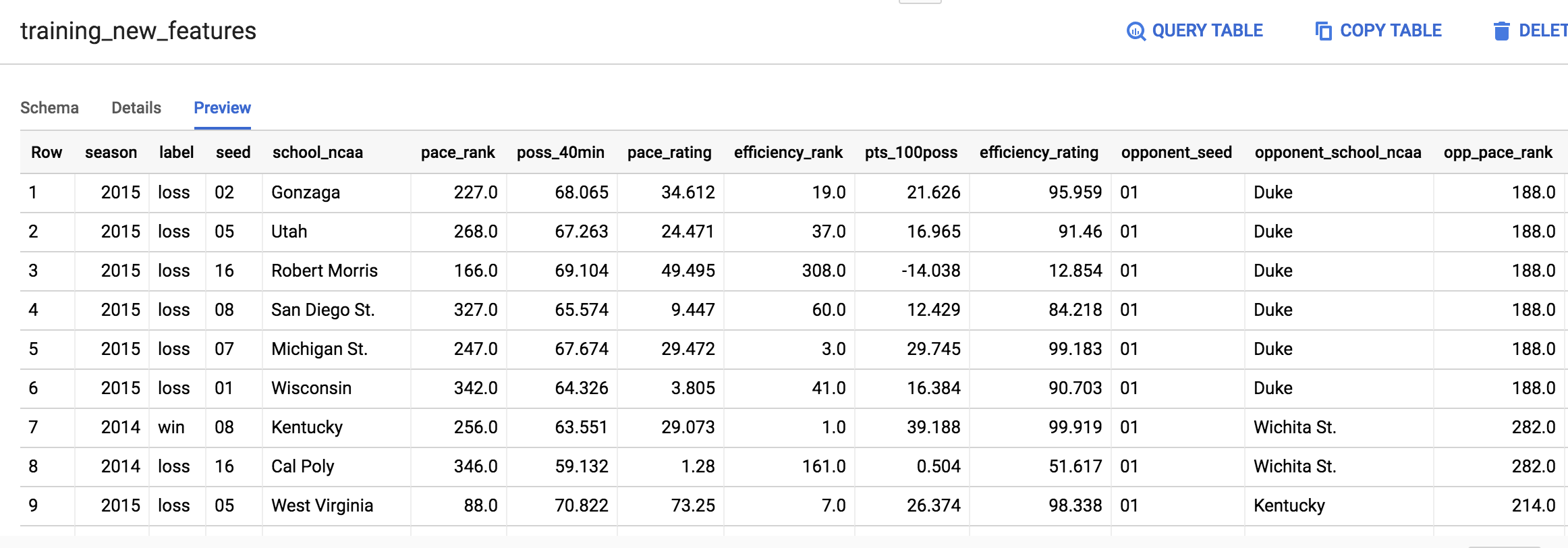
Don't worry if your output is not identical to the above screenshot.

Task 14. Interpreting selected metrics

• You will now learn about some important labels that aid us in making predictions.

opp_efficiency_rank

Opponent's Efficiency Rank: out of all the teams, what rank does our opponent have for scoring efficiently over time (points per 100 basketball possessions). Lower is better.

opp_pace_rank

Opponent's Pace Rank: out of all teams, what rank does our opponent have for basketball possession (number of possessions in 40 minutes). Lower is better.

Now that you have insightful features on how well a team can score and how well it can hold on to the basketball lets train our second model.

As an additional measure to safe-guard your model from "memorizing good teams from the past", exclude the team's name and the seed from this next model and focus only on the metrics.

Task 15. Train the new model

• Run the following command in the query EDITOR:

CREATE OR REPLACE MODEL
  `bracketology.ncaa_model_updated`
OPTIONS
  ( model_type='logistic_reg') AS

SELECT
  # this time, don't train the model on school name or seed
  season,
  label,

  # our pace
  poss_40min,
  pace_rank,
  pace_rating,

  # opponent pace
  opp_poss_40min,
  opp_pace_rank,
  opp_pace_rating,

  # difference in pace
  pace_rank_diff,
  pace_stat_diff,
  pace_rating_diff,


  # our efficiency
  pts_100poss,
  efficiency_rank,
  efficiency_rating,

  # opponent efficiency
  opp_pts_100poss,
  opp_efficiency_rank,
  opp_efficiency_rating,

  # difference in efficiency
  eff_rank_diff,
  eff_stat_diff,
  eff_rating_diff

FROM `bracketology.training_new_features`

# here we'll train on 2014 - 2017 and predict on 2018
WHERE season BETWEEN 2014 AND 2017 # between in SQL is inclusive of end points

Soon after, your output should look similar to the following:

Task 16. Evaluate the new model's performance

• To evaluate your model's performance, run the following command in the query EDITOR:

SELECT
  *
FROM
  ML.EVALUATE(MODEL     `bracketology.ncaa_model_updated`)

Your output should look similar to the followings:

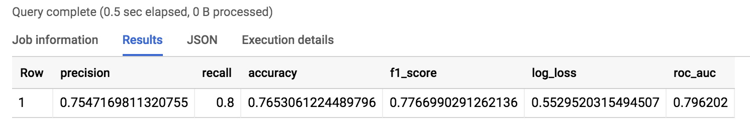
Wow! You just trained a new model with different features and increased your accuracy to around 75% or a 5% lift from the original model.

This is one of the biggest lessons learned in machine learning is that your high quality feature dataset can make a huge difference in how accurate your model is.

Click Check my progress to verify the objective.

Train the new model and make evaluation

Check my progress

Task 17. Inspect what the model learned

• Which features does the model weigh the most in win / loss outcome? Find out by running the following command in the query EDITOR:

SELECT
  *
FROM
  ML.WEIGHTS(MODEL     `bracketology.ncaa_model_updated`)
ORDER BY ABS(weight) DESC

Your output should look like this:

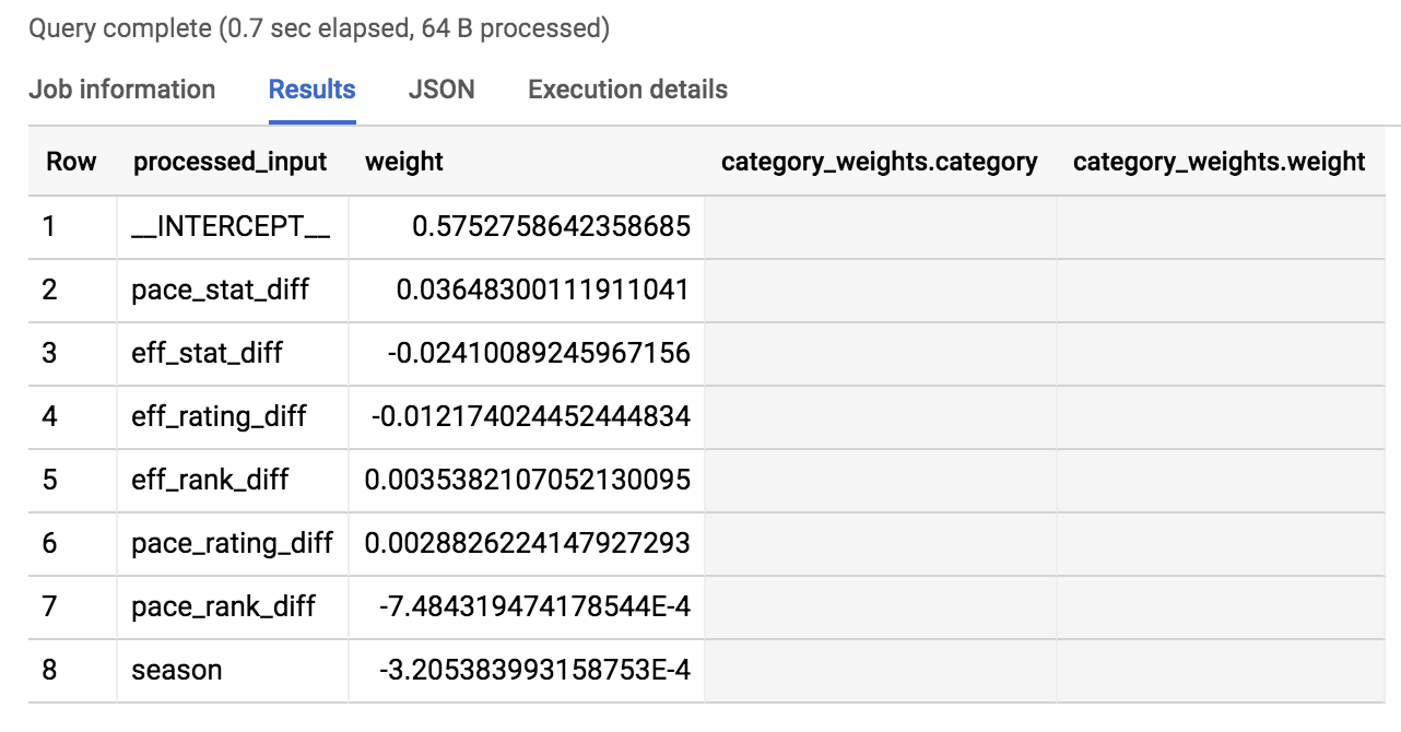
We've taken the absolute value of the weights in our ordering so the most impactful (for a win or a loss) are listed first.

As you can see in the results, the top 3 are pace_stat_diff, eff_stat_diff, and eff_rating_diff. Let's explore these a little bit more.

pace_stat_diff

How different the actual stat for (possessions / 40 minutes) was between teams. According to the model, this is the largest driver in choosing the game outcome.

eff_stat_diff

How different the actual stat for (net points / 100 possessions) was between teams.

eff_rating_diff

How different the normalized rating for scoring efficiency was between teams.

What did the model not weigh heavily in its predictions? Season. It was last in the output of ordered weights above. What the model is saying is that the season (2013, 2014, 2015) isn't that useful in predicting game outcome. There wasn't anything magical about the year "2014" for all teams.

An interesting insight is that the model valued the pace of a team (how well they can control the ball) over how efficiently a team can score.

Task 18. Prediction time!

• Run the following command in the query EDITOR:

CREATE OR REPLACE TABLE `bracketology.ncaa_2018_predictions` AS

# let's add back our other data columns for context
SELECT
  *
FROM
  ML.PREDICT(MODEL     `bracketology.ncaa_model_updated`, (

SELECT
* # include all columns now (the model has already been trained)
FROM `bracketology.training_new_features`

WHERE season = 2018

))

Your output should be similar to the following:

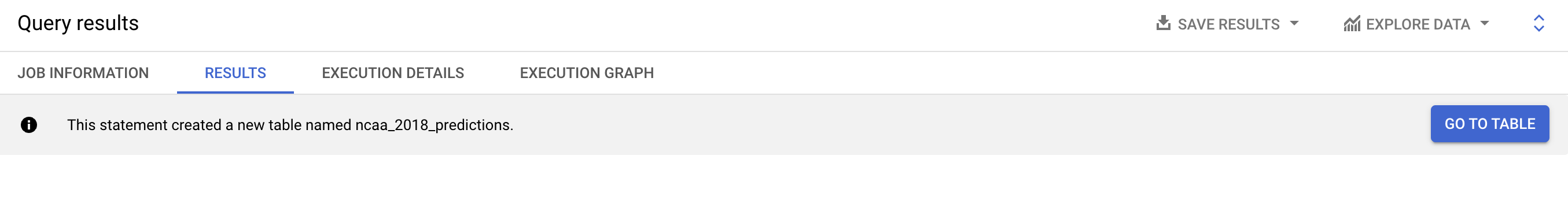
Click Check my progress to verify the objective.

Run a query to create a table ncaa_2018_predictions

Check my progress

Task 19. Prediction analysis:

Since you know the correct game outcome, you can see where your model made an incorrect prediction using the new testing dataset.

• Run the following command in the query EDITOR:

SELECT * FROM `bracketology.ncaa_2018_predictions`
WHERE predicted_label <> label

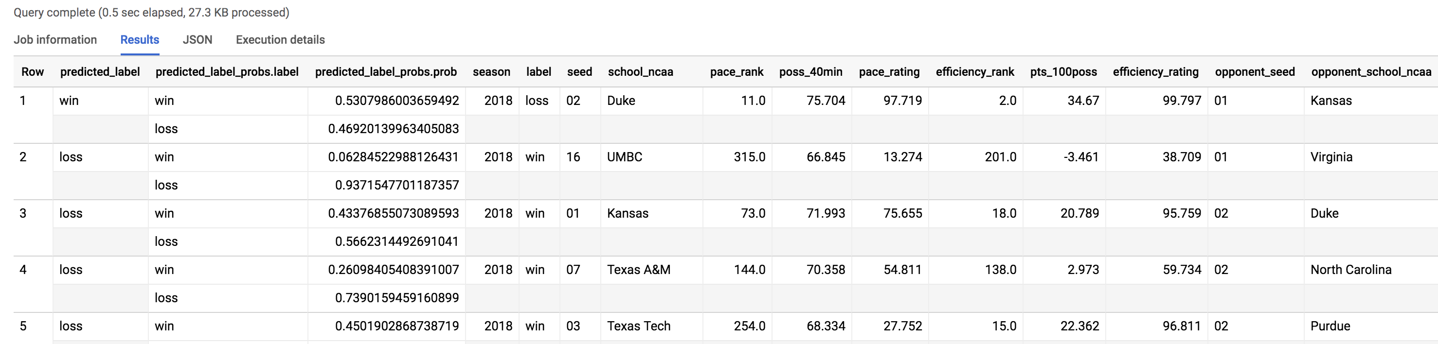
As you can see from the number of records returned from the query, the model got 48 matchups wrong (24 games) out of the total number of matchups in the tournament for a 2018 accuracy of 64%. 2018 must have been a wild year, let's look at what upsets happened.

Task 20. Where were the upsets in March 2018?

• Run the following command in the query EDITOR:

SELECT
CONCAT(school_ncaa, " was predicted to ",IF(predicted_label="loss","lose","win")," ",CAST(ROUND(p.prob,2)*100 AS STRING), "% but ", IF(n.label="loss","lost","won")) AS narrative,
predicted_label, # what the model thought
n.label, # what actually happened
ROUND(p.prob,2) AS probability,
season,

# us
seed,
school_ncaa,
pace_rank,
efficiency_rank,

# them
opponent_seed,
opponent_school_ncaa,
opp_pace_rank,
opp_efficiency_rank

FROM `bracketology.ncaa_2018_predictions` AS n,
UNNEST(predicted_label_probs) AS p
WHERE
  predicted_label <> n.label # model got it wrong
  AND p.prob > .75  # by more than 75% confidence
ORDER BY prob DESC

Your outcome should look like:

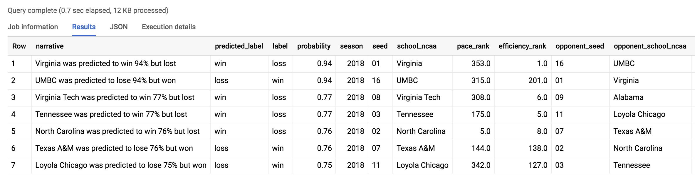
The major upset was the same one our previous model found: UMBC vs Virginia. Read more about how 2018 overall was a year of huge upsets in Has This Been the “Maddest” March? article. Will 2019 be just as wild?

Task 21. Comparing model performance

What about where the naive model (comparing seeds) got it wrong but the advanced model got it right?

• Run the following command in the query EDITOR:

SELECT
CONCAT(opponent_school_ncaa, " (", opponent_seed, ") was ",CAST(ROUND(ROUND(p.prob,2)*100,2) AS STRING),"% predicted to upset ", school_ncaa, " (", seed, ") and did!") AS narrative,
predicted_label, # what the model thought
n.label, # what actually happened
ROUND(p.prob,2) AS probability,
season,

# us
seed,
school_ncaa,
pace_rank,
efficiency_rank,

# them
opponent_seed,
opponent_school_ncaa,
opp_pace_rank,
opp_efficiency_rank,

(CAST(opponent_seed AS INT64) - CAST(seed AS INT64)) AS seed_diff

FROM `bracketology.ncaa_2018_predictions` AS n,
UNNEST(predicted_label_probs) AS p
WHERE
  predicted_label = 'loss'
  AND predicted_label = n.label # model got it right
  AND p.prob >= .55  # by 55%+ confidence
  AND (CAST(opponent_seed AS INT64) - CAST(seed AS INT64)) > 2 # seed difference magnitude
ORDER BY (CAST(opponent_seed AS INT64) - CAST(seed AS INT64)) DESC

Your outcome should look like:

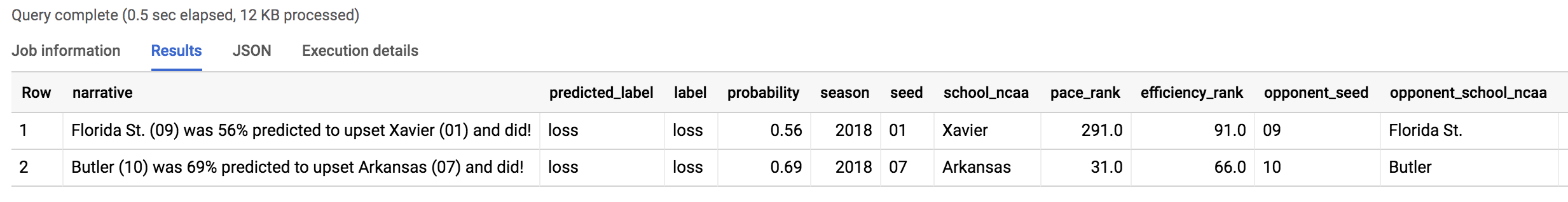
The model predicted a Florida St. (09) upset of Xavier (01) and they did!

The upset was correctly predicted by the new model (even when the seed ranking said otherwise) based on your new skillful features like pace and shooting efficiency. Watch the game highlights on YouTube.

Task 22. Predicting for the 2019 March Madness tournament

Now that we know the teams and seed rankings for March 2019, let's predict the outcome of future games.

Explore the 2019 data

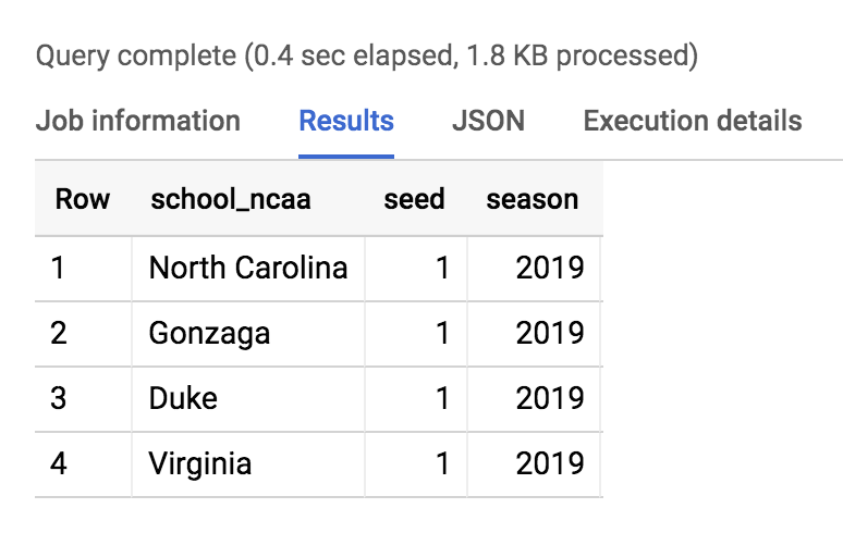
• Run the below query to find the top seeds

SELECT * FROM `data-to-insights.ncaa.2019_tournament_seeds` WHERE seed = 1

Your outcome should look like:

Create a matrix of all possible games

Since we don't know which teams will play each other as the tournament progresses, we'll simply have them all face each other.

In SQL, an easy way to have a single team play every other team in a table is with a CROSS JOIN.

• Run the below query to get all possible team games in the tournament.

SELECT
  NULL AS label,
  team.school_ncaa AS team_school_ncaa,
  team.seed AS team_seed,
  opp.school_ncaa AS opp_school_ncaa,
  opp.seed AS opp_seed
FROM `data-to-insights.ncaa.2019_tournament_seeds` AS team
CROSS JOIN `data-to-insights.ncaa.2019_tournament_seeds` AS opp
# teams cannot play against themselves :)
WHERE team.school_ncaa <> opp.school_ncaa

Add in 2018 team stats (pace, efficiency)

CREATE OR REPLACE TABLE `bracketology.ncaa_2019_tournament` AS

WITH team_seeds_all_possible_games AS (
  SELECT
    NULL AS label,
    team.school_ncaa AS school_ncaa,
    team.seed AS seed,
    opp.school_ncaa AS opponent_school_ncaa,
    opp.seed AS opponent_seed
  FROM `data-to-insights.ncaa.2019_tournament_seeds` AS team
  CROSS JOIN `data-to-insights.ncaa.2019_tournament_seeds` AS opp
  # teams cannot play against themselves :)
  WHERE team.school_ncaa <> opp.school_ncaa
)

, add_in_2018_season_stats AS (
SELECT
  team_seeds_all_possible_games.*,
  # bring in features from the 2018 regular season for each team
  (SELECT AS STRUCT * FROM `data-to-insights.ncaa.feature_engineering` WHERE school_ncaa = team AND season = 2018) AS team,
  (SELECT AS STRUCT * FROM `data-to-insights.ncaa.feature_engineering` WHERE opponent_school_ncaa = team AND season = 2018) AS opp

FROM team_seeds_all_possible_games
)

# Preparing 2019 data for prediction
SELECT

  label,

  2019 AS season, # 2018-2019 tournament season

# our team
  seed,
  school_ncaa,
  # new pace metrics (basketball possession)
  team.pace_rank,
  team.poss_40min,
  team.pace_rating,
  # new efficiency metrics (scoring over time)
  team.efficiency_rank,
  team.pts_100poss,
  team.efficiency_rating,

# opposing team
  opponent_seed,
  opponent_school_ncaa,
  # new pace metrics (basketball possession)
  opp.pace_rank AS opp_pace_rank,
  opp.poss_40min AS opp_poss_40min,
  opp.pace_rating AS opp_pace_rating,
  # new efficiency metrics (scoring over time)
  opp.efficiency_rank AS opp_efficiency_rank,
  opp.pts_100poss AS opp_pts_100poss,
  opp.efficiency_rating AS opp_efficiency_rating,

# a little feature engineering (take the difference in stats)

  # new pace metrics (basketball possession)
  opp.pace_rank - team.pace_rank AS pace_rank_diff,
  opp.poss_40min - team.poss_40min AS pace_stat_diff,
  opp.pace_rating - team.pace_rating AS pace_rating_diff,
  # new efficiency metrics (scoring over time)
  opp.efficiency_rank - team.efficiency_rank AS eff_rank_diff,
  opp.pts_100poss - team.pts_100poss AS eff_stat_diff,
  opp.efficiency_rating - team.efficiency_rating AS eff_rating_diff

FROM add_in_2018_season_stats

Make predictions

CREATE OR REPLACE TABLE `bracketology.ncaa_2019_tournament_predictions` AS

SELECT
  *
FROM
  # let's predicted using the newer model
  ML.PREDICT(MODEL     `bracketology.ncaa_model_updated`, (

# let's predict on March 2019 tournament games:
SELECT * FROM `bracketology.ncaa_2019_tournament`
))

Click Check my progress to verify the objective.

Run queries to create tables ncaa_2019_tournament and ncaa_2019_tournament_predictions

Check my progress

Get your predictions

SELECT
  p.label AS prediction,
  ROUND(p.prob,3) AS confidence,
  school_ncaa,
  seed,
  opponent_school_ncaa,
  opponent_seed
FROM `bracketology.ncaa_2019_tournament_predictions`,
UNNEST(predicted_label_probs) AS p
WHERE p.prob >= .5
AND school_ncaa = 'Duke'
ORDER BY seed, opponent_seed

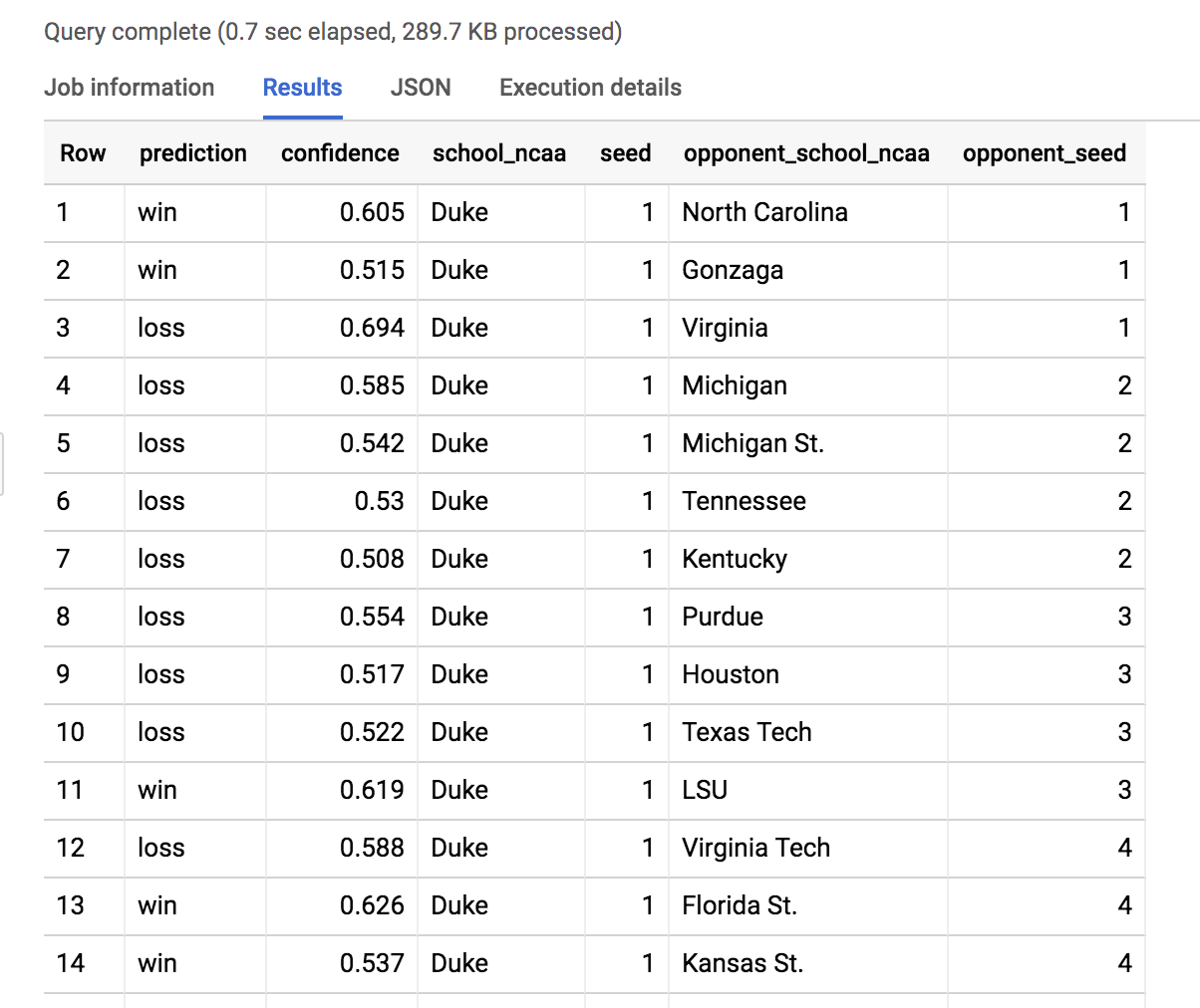
• Here we filtered the model results to see all of Duke's possible games. Scroll to find the Duke vs North Dakota St. game.

Insight: Duke (1) is 88.5% favored to beat North Dakota St. (16) on 3/22/19.

Experiment by changing the school_ncaa filter above to predict for the matchups in your bracket. Write down what the model confidence is and enjoy the games!

---

Solution of Lab

curl -LO raw.githubusercontent.com/ePlus-DEV/storage/refs/heads/main/labs/export-data-from-big-query-to-cloud-storage/lab.sh
source lab.sh

Script Alternative

curl -LO raw.githubusercontent.com/QUICK-GCP-LAB/2-Minutes-Labs-Solutions/main/Bracketology%20with%20Google%20Machine%20Learning/gsp461.sh
sudo chmod +x gsp461.sh
./gsp461.sh